This tutorial will show you how to export the results of your analysis. This allows users to report specific signals, metrics, or events from a data set and to share results from analysis conducted within Inspect3D.

This tutorial uses overground walking data from four subjects. The subjects walked at three different speeds: slow, normal and fast. The data was processed using a pipeline with automatic event detection and link model based item calculations (most notably the knee joint angles). Four Subjects Walking Data Set].

This tutorial also uses query definitions that have been previously saved in a .q3d file. AnkleAngles.q3d].

As with previous tutorials, we begin by loading the library and defining the queries relevant to our question.

1. Click Load Library in the toolbar to open the Load Library dialog.

2. Click Browse and select the folder where the data is stored.

3. Click Load button to import the data.

For this tutorial we will load previously saved query definitions and use them to calculate our specific groups.

1. Click on the Query Definitions icon on the toolbar and then click on Load Query Def & Compute Groups.

2. Select the AnkleAngles.q3d file with the saved query definitions and Open them.

Three groups will now appear in the Groups list: ANKLE_ANGLE_X, ANKLE_ANGLE_Y, and ANKLE_ANGLE_Z. Clicking on any of the groups will show that each of the four workspaces is associated with that group.

We can visualize the groups individually and collectively in different plots in the Queried Data area. For a full overview of how to visualize data, see the tutorial. 1. To start, click on Show Options.

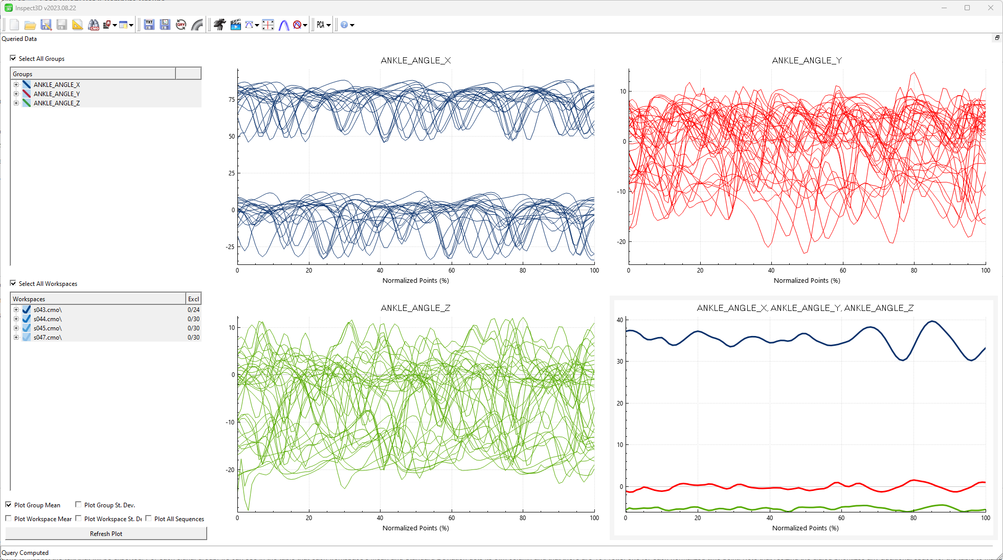
2. Under Plotting options choose 2 Graph Rows and 2 Graph Columns to create a 2×2 set of plots in the Queried Data area.

3. Close the Show Options dialog.

4. With the top-left plot selected (this will be indicated with a light-grey border), select the ANKLE_ANGLE_X group, select all workspaces, and then plot the raw sequences.

5. Select the top-right plot and plot the raw sequences from the ANKLE_ANGLE_Y group's workspaces.

6. Select the bottom-left plot and plot the raw sequences from the ANKLE_ANGLE_Z group's workspaces.

7. Select the bottom-right plot, select all groups and all workspaces, and plot the group means.

It is possible now to export the visualizations to one of four image formats: JPG, PDF vector graphic, PNG, or BMP. 1. Right-click the bottom-right plot and select Export Graph… from the context menu.

2. In the Export Graph dialog, choose your desired Export Path, leave Use Current Size checked, and set the Format to “.pdf (vector graphics)”.

3. Click Save.

4. Alternatively, export all four graphs collectively by selecting Export Graphs on the toolbar.

5. In the Export Graph dialog, choose your desired Export Path, uncheck Use Current Size, specify Height and Width to be 400 pixels each, and set the Format to “.jpg”.

Alternatively, we can export our signal data to a text format. 1. Click Export Results on the application toolbar.

2. In the Export Results dialog's Definition section, set the Export Type to Signals, the Input Data to All Queried Data, and select both Workspace Mean and Workspace Std. Dev..

3. In the Export Results dialog's Export Result Options section, leave the default Export Format and Precision and click Generate Preview.

4. The Table of results will populate and you can scroll in both directions to inspect the text that will be exported. For each signal group, we can see in the table that each Workspace's Mean and Standard Deviation gets its own column and that there are 101 rows, one for each normalized time point. Note that resizing the dialog prioritizes any additional space for the table to make it easier to view large output files.

5. Specify a Results File Name and then click Export Results to finalize the export.

We can also export metrics based on the data to a text format.

1. Returning to the Export Results dialog's Definition section, set the Export Type to Metrics, set Calculate results for to Workspaces, and select both Minimum and Maximum.

2. In the Export Results dialog's Export Result Options section, click Generate Preview. For each signal group, we can see that the table contains each workspace's minimum mean value and maximum mean value.

3. Back in the main application window, click on the top-left plot.

4. In the Export Results dialog's Definition section, set Input Data to Active Plot Data

5. Click Generate Preview again. Now we can see that our selected metrics (Minimum and Maximum) will only be exported to the ANKLE_ANGLE_X traces, since this is the data on the currently active plot.

6. Specify a Results File Name and then click Export Results to finalize the export.

In order to export Principal Component Analysis (PCA)results, we have to first calculate the PCA results! For a full overview of how to perform PCA and interpret some of the results, see the tutorial.

1. Ensure that all groups and workspaces are selected in the Groups and Workspaces lists.

2. Open the PCA Options dropdown menu on the toolbar.

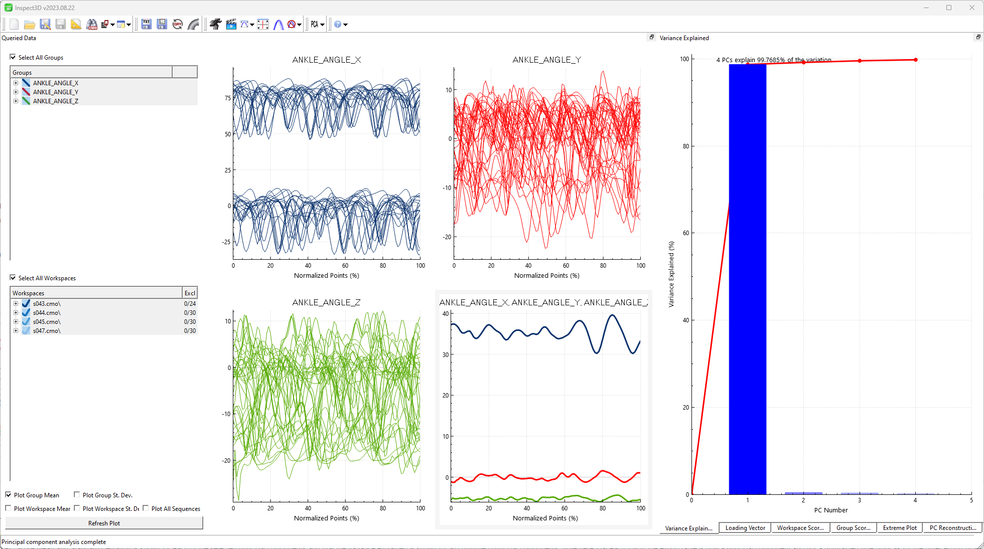
3. Set Number PCs to 4 and ensure that Use Workspace Mean is checked.

4. Click Run PCA.

5. The results of these calculations will automatically populate the PCA graphs. If these aren't already displayed, click Show PCA Graphs in the PCA Options dropdown menu. Because the traces for each signal cluster around a distinctive mean value, almost all of the variance in these groups can be captured by a single principal component.

Now that we have performed PCA, we have results to export. 1. Click Export Results on the application toolbar.

2. In the Export Results dialog's Definition section, set the Export Type to PCA Results and select the Group Scores, Group Scores Std. Dev., and Variance Explained options.

3. In the Export Results dialog's Export Result Options section, leave Export Format as Standard ASCII and Precision as 4.

4. Click Generate Preview. We can see that each signal's Group PC Score Mean and Standard Deviation is shown for each of the selected principal components and that the variance explained is shown for all computed principal components. Note here that each row in the export table is now a principal component and not a normalized time point as for the other export types. Also note that Inspect3D does have the ability to export information about all of the principal components that were calculated, not only the ones that were selected.

In this tutorial you learned how to export the traces visualized in Inspect3D to common image formats. You also learned how to export three types of data to text: Signals, Metrics, and PCA Results.

Previous: Tutorial 3: Perform Principal Component Analysis

Inspect3D Getting Started Tutorials

Next: Finished!