The mathematical principles of PCA presented here are drawn from Chapter 14 of the Research Methods in Biomechanics textbook ¹⁾.

New technology allows researchers to generate large quantities of data, whether it be time-series data, or any other waveform data that we commonly see in biomechanics research. And what is common among all these forms of data is that they are highly dimensional ¹⁾. With technologies like markerless motion capture, inertial measurement units, and EMG, researchers are collecting so much data that making meaningful comparisons is difficult conceptually and computationally. The authors of Research Methods in Biomechanics emphasize that the basic point of dimensionality reduction for biomechanical waveforms is that no matter the research questions that a biomechanist is asking, reducing the dimensionality of our data generally makes it more manageable and useful for analysis ¹⁾. Traditional approaches for extracting features from waveform data include spatiotemporal features such as maximums, minimums, and ranges, etc. but this style of summary results in a loss of information available for follow-on analysis. Additionally, varying definitions for these discrete parameters across the field lead to inconsistent conclusions and these parameters may not always be definitive in certain populations ¹⁾. One such example is that knee adduction angles in patients with OA don’t have definitive peaks making it an ill-defined problem to find maximum and minimum angles across gait cycles ²⁾.

There is a lot of structure in biomechanical waveforms and this is especially true of kinematic variables such as joint angles. These waveforms are often smooth and have gradual rates-of-change. This means that if we know the value of a kinematic variable at one point in time, we have a very good idea of which neighbourhood the values will be found in for nearby points in time. As a result, we don't need all of the data points in a waveform to have a very good idea of the waveform as a whole.

PCA is a principled way of reducing the dimensionality of data with minimal information lost regarding the data set's variability. Put technically, PCA is an orthogonal decomposition technique that computes and extracts a unique set of basis functions from the waveforms based on the variation that is present in the waveform data ¹⁾. In practice, we can often reduce a 101-dimensional waveform (typical of time-normalized waveforms) to 4 or 5 dimensions while retaining information about more than 90% of the data set's variability. This can help us avoid the curse of dimensionality for follow-on analysis.

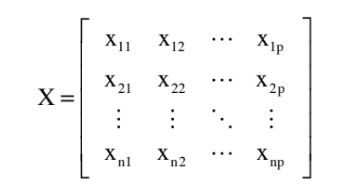
Waveform data can be represented in matrix form , where the rows are the time series waveforms for each subject and the columns are particular points within the waveform (n = subjects, p = points) ¹⁾.

Note that representing our waveforms as a matrix requires us to time-normalize the waveforms so that they are all of the same length (that they contain the same number of points). Sift is capable of computing PCA for time-normalized waveforms where there is |DATA_NOT_FOUND but will produce a warning message that cautions the user to interpret the results with care.

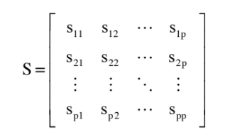
Variation in the waveform matrix, X, is based on how the data changes between subjects (n) at each point in time (p). Mathematically this variance is represented by the covariance matrix, S. The diagonal elements of the covariance matrix are the variation at each instance in the data. The off-diagonal elements represent the variation in each pair of instances. Non-zero covariance values mean that the columns of the original data matrix X are correlated.

Since we want to find principal components that are orthogonal, we need to transform our covariance matrix, S, into a new covariance matrix, D, where the off-diagonal components are equal to zero ¹⁾. This transformation is accomplished using diagonalization, where U is an orthogonal transformation matrix. U transforms the data into the new coordinate system, which are the coordinates of the principal components ¹⁾.

U'SU = D

The columns of matrix U are the eigenvectors of the covariance matrix S. Many people refer to these eigenvectors as the principal component's loading vectors ¹⁾.

The matrix D is a diagonal covariance matrix. The individual elements of D are the individual measures of variance for each principal component, and are the eigenvalues of the covariance matrix S ¹⁾.

See also the PCA module's Loading Vector graph.

Finally, we use the matrix U to transform our original data matrix X into orthogonal principal components (uncorrelated) ¹⁾. Since the principal components of a data set are independent of that data set's mean values, we subtract the mean values of X before this transformation.

The columns of Z are the principal components (linear combinations of the underlying waveform data), while the individual components are the PC scores ¹⁾.

Z = U'XU

See also the PCA module's Workspace Scores and Group Scores graphs.

The diagonal elements of D, the eigenvalues, give the variance of each PC. The total variance explained by our principal components is the sum of these diagonal elements which is called the matrix's trace (tr) ¹⁾.

tr(S)=tr(D)

The variance explained by an individual PC is then the ratio between that PC's eigenvalue and the trace of the matrix.

See also the PCA module's Variance Explained graph.