This tutorial will show you how to use the outlier detection methods built into Sift, when each method might be appropriate and how to interpret the results. Outlier detection is a key artifact of data analysis, identifying errant data or anomalies that might make further data analysis less effective. Within Sift, there are multiple methods for detecting outliers, but we will be focusing on doing so with PCA data in this tutorial.

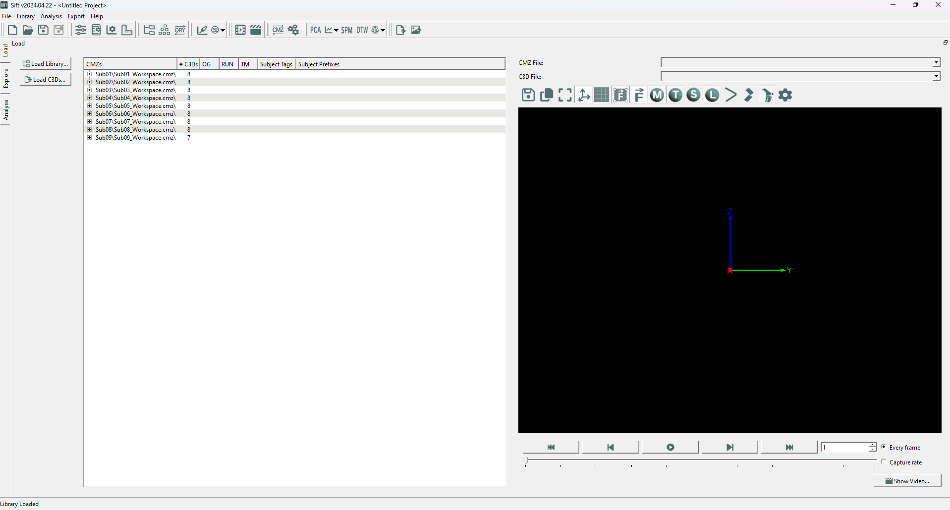
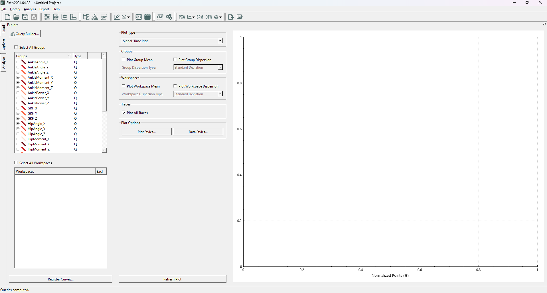
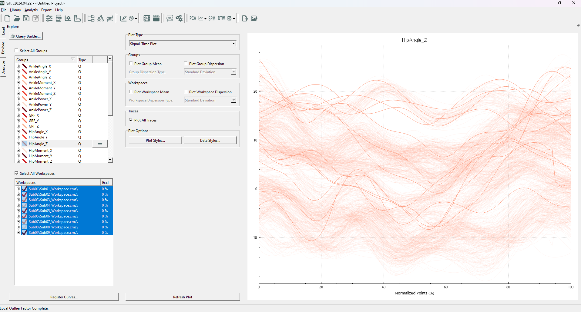
For this tutorial, we will be examining some gait data from a Visual3D Workshop at a recent ASB meeting. We first need to load the .CMZs into Sift (load from the V3D Workshop folder), and then create and calculate some queries. We will simply use the results from Sifts built in Auto Populate Queries dialog. Your load and explore pages should look as follows:

If you are having trouble with the above instructions, the Sift Tutorials wiki page has many tutorials that will help you out.

Local Outlier Factor(LOF) is a outlier detection method that uses the local density around data points to determine if a point is an outlier. In this sense it can find outliers that global detection methods would not, as it identifies outliers in local areas.

In Sift, LOF is built upon the PCA module, to find outliers in the PC workspace scores. As such, we will need to create a PCA analysis. To show the benefits of Local Outlier Factor, we will be using the group “HipAngle_Z”, as it has a good shape to demonstrate the effectiveness of LOF (multiple clusters of varying density). Specifically, create a PCA with:

• HipAngle_Z selected (and all workspaces)
• 4 PCs calculated
• “Use Workspace Mean” unchecked
• Named “PCA_HipZ”

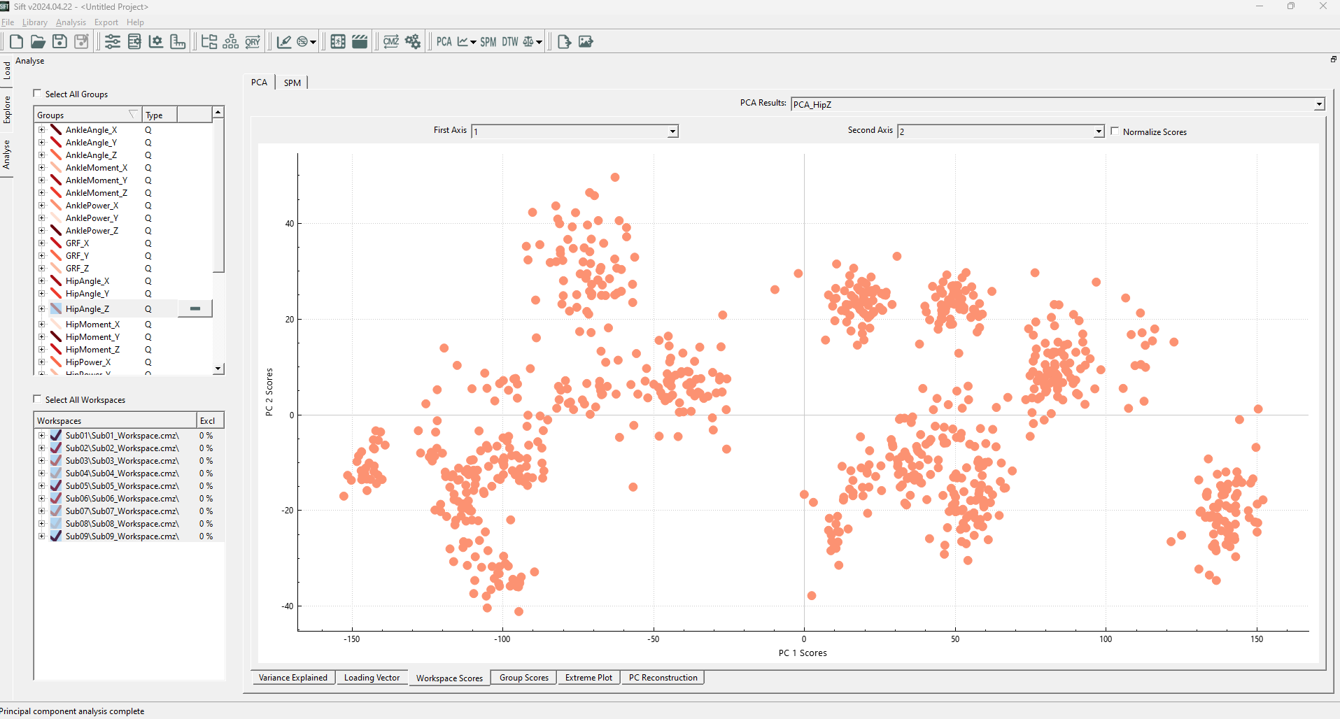
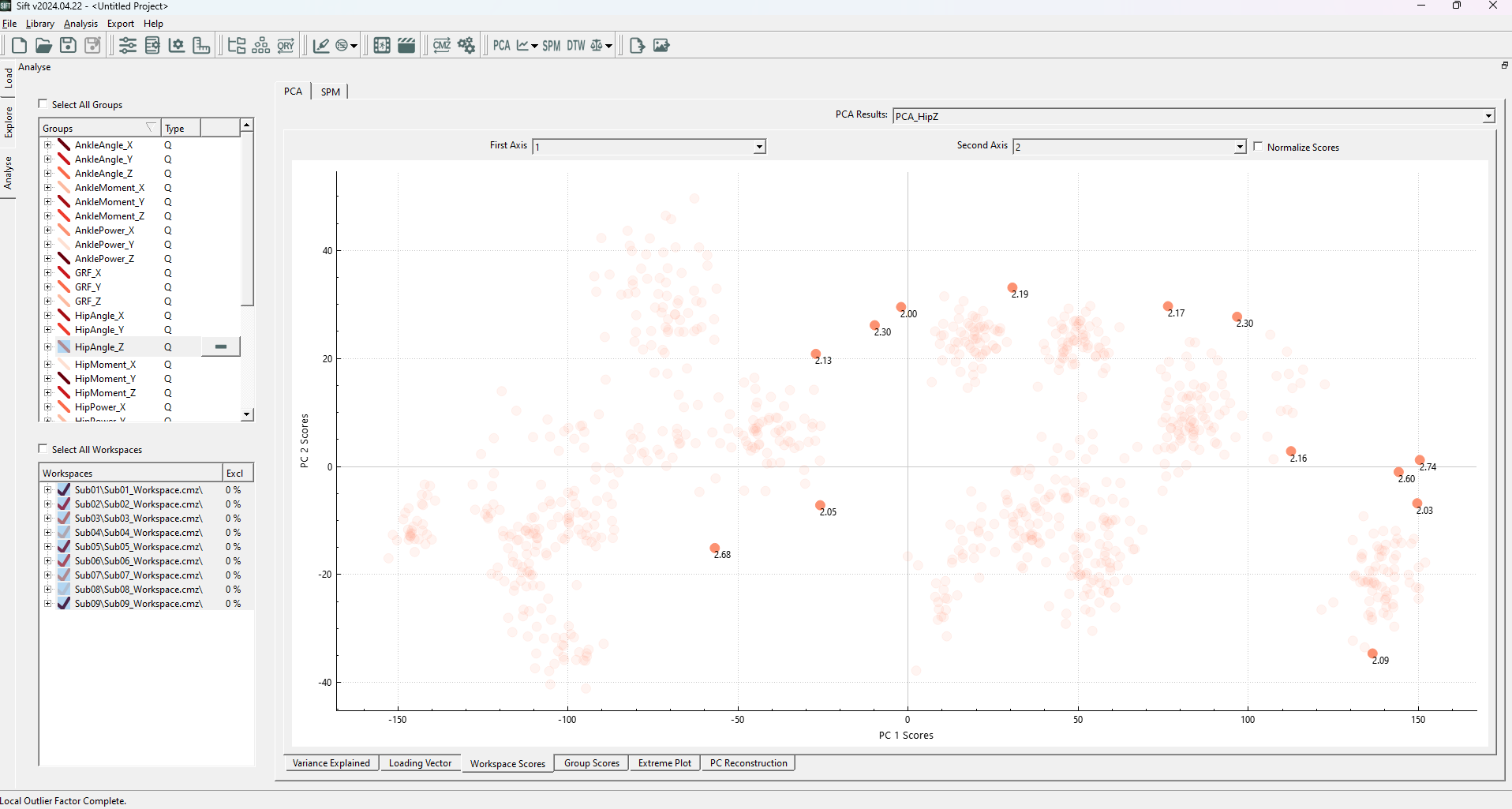
After calculating the PCA Results, the Workspace Scores on the analyse page should look as follows (note that the points are coloured by group. If they were coloured by workspace, you would see many of these clusters correspond to workspaces):

We can see several distinct clusters, in varying positions (and none of which are located at the origin of the plot!). This could cause issues if we were to use “global” outlier detection methods: individual data points may appear to be inliers globally but are actually locally an outlier (i.e. if it is between but not in any of several clusters), or vice-versa, a point (or cluster of points) may be at the edge of the global distribution, but well within a local cluster distribution.

Whichever the situation may be, we are interested in finding outliers in our data, and making a decision upon finding them. We will start by running a LOF calculation. To do so, open the Outlier Detection Using PCA dropdown on the toolbar, and select “Local Outlier Factor”.

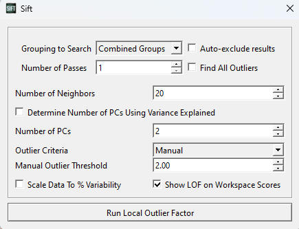
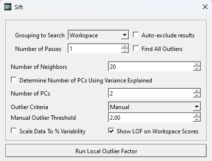
A pop-up window will appear, allowing you to customize some features of the LOF calculation. For this first test, we should set the parameters as below (in the image):

For now, we are looking for outliers from within the entire PCA analysis. We could partition it such that points only calculate their LOF against points in their own group or workspace (which we will show later), but for now we want to look at the whole graph as one, and as such we have selected “Combined Groups”.

The number of neighbors is a tuneable parameter within the LOF calculation, and determines how large of a local grouping we will look at. According to the original paper introducing LOF, a k-value below ~10 can cause issues, so we will at least choose this. They also recommend choosing a k of at least the minimum number of points in a cluster. Looking through our data, a k value >= 20 seems reasonable, so we will use k=20.

We choose to use 2 PCs, as the workspace scores are presented in 2 dimensions.

Lastly, we choose a manual threshold of 2.0. There is no specific rule for choosing a threshold for inliers vs. outliers, but it should be a number > 1, as below 1 is classified as an inlier. Through iteration, 2.0 is a reasonable value for this data set, as we will see. Generally, we have found that thresholds should be at least > 1.5 to be useful, and to not exclude inliers.

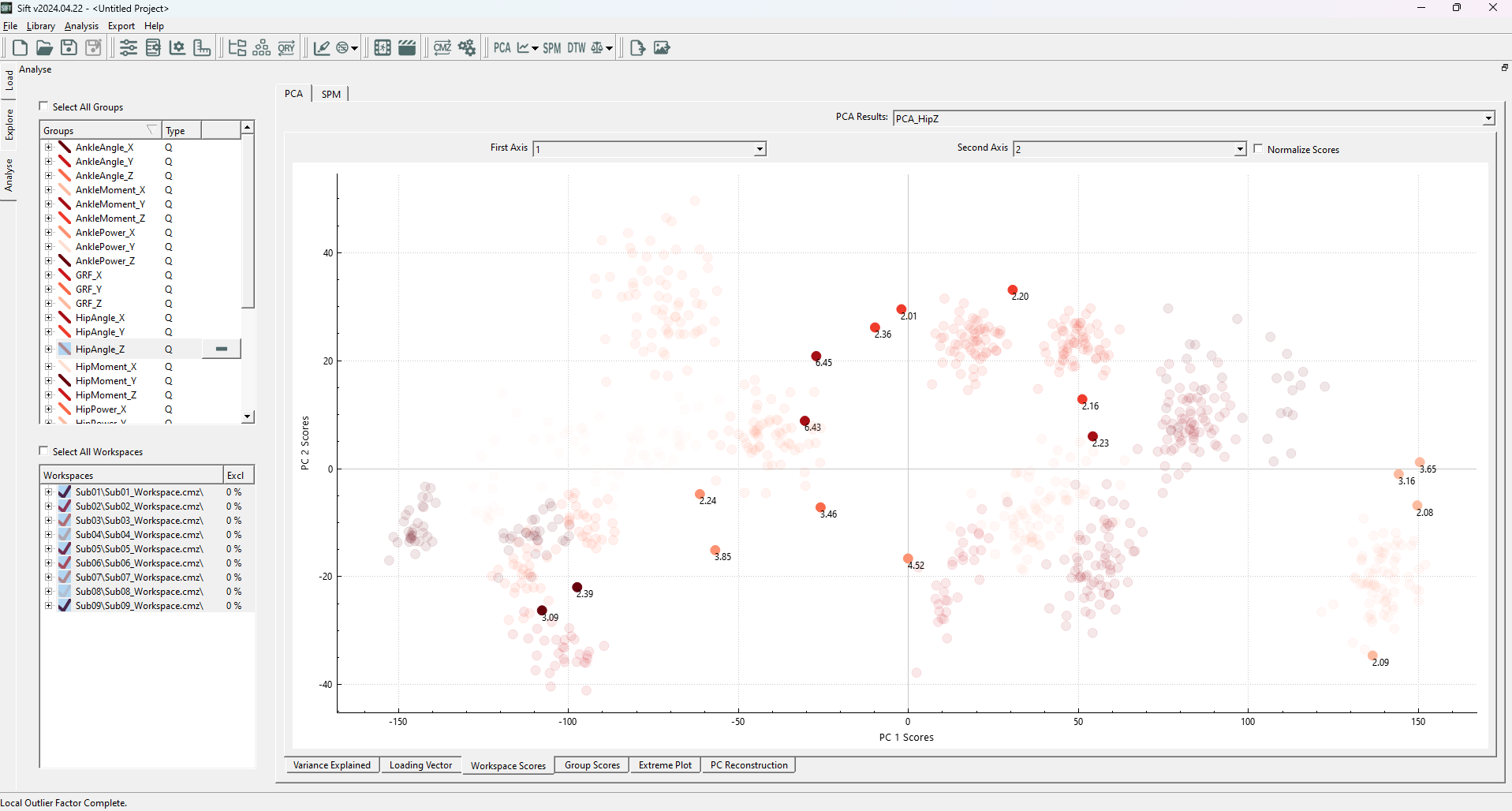
Upon running the LOF analysis, you should see several datapoints highlighted:

The highlighted points generally follow what we were hoping to see, any points outside of local clusters are identified as outliers. We see that inliers are determined as such regardless of their cluster density (ex the cluster in the top left is much less dense than others, but is still a valid cluster). We can observe that many of these traces (in the explore page) do not necessarily follow the same trends as the rest of the data, and conclude that they are outliers.

Because Sift has automatically selected the values identified to be outliers, we can easily exclude them on the explore page (if we didn't already do so through the LOF dialog). Simply right click on the explore page graph, and select exclude→exclude data (raw traces). To instead deselect the outlier traces, hit ctrl+h on your keyboard, and you should see the all traces highlighted (including their LOF values in the workspace scores graph).

Before doing different analysis, we will want to reset our change. To re-include the data (if you have excluded it), right click on the workspaces dialog on the left, and select re-include all data.

Another way we might want to examine the data is by comparing the data to only their own workspace. Maybe one of the traces was abnormal for that person (and should be removed), but it looks similar to that of another workspace. With combined groups this might not be identified as an outlier. We thus alter the LOF dialog to be as so:

Note that we have left the other parameters the same, as we still think k=20 is a reasonable number of neighbors. Upon running this analysis we see a slightly different section of datapoints chosen (note that the graph is coloured by workspace now as opposed to group):

Here we notice that (among others) several points in the bottom left side are selected as outliers, and several points that were initially identified as outliers in the top right no longer are. The reason for both of these is simply that they are/aren't outliers in different contexts. The new outliers belong to a workspace for which most data points are not in the immediate local area, even though data points from other workspaces are in the local area. Similarly, the new inliers in the top right are determined to be inliers because when workspaces were combined, multiple workspaces overlapped in that local area, increasing the density for their neighbors. Some of these points were only marginally determined to be outliers (close to a score of 2), which could represent that the threshold value of 2.0 was a little low.

Automatically finding outliers saves time and effort, and can lead to more objective results, if it is done based on some criteria or test. There are very simple methods that could be employed, like finding the data that is farthest away from the mean and excluding some portion of those, or those that are further than some distance away. As we see in the Mahalanobis Distance , the distance measure we use can be very important: Data may be located close to the mean data, but outlying in comparison to the general trend of the data, or it may be located far from the mean data, but in line with the trend and just towards an upper limit along an axis. The Mahalanobis Distance Test is an outlier detection method that uses the underlying covariance relationship of data to determine outliers which don't follow the general trend of the data. In conjunction with the Mahalanobis Distance test, we also have the Squared Prediction Error. This is a test which measures how far a prediction is from the real data, or in this case, how far our PC-decomposed representation is from the real data. These 2 methods work well together: we can measure how close a single prediction follows the general trend, and we can measure how a single prediction compares to the ground truth. This is why we have bundled them together in Sift.

In Sift, both methods also built upon the PCA module, to find outliers in the PC workspace scores. As such, we will need to create a PCA analysis. To show the benefits of Mahalanobis Distance Test and SPE, we will be using the group “HipPower_X”, as it has a good shape to demonstrate the effectiveness of Mahalanobis Distance Tests (most data following a specific trend, with some close by outliers not following the same trend). Specifically, create a PCA with:

• HipPower_X selected (and all workspaces)
• 4 PCs calculated
• “Use Workspace Mean” unchecked
• Named “PCA_HipX”

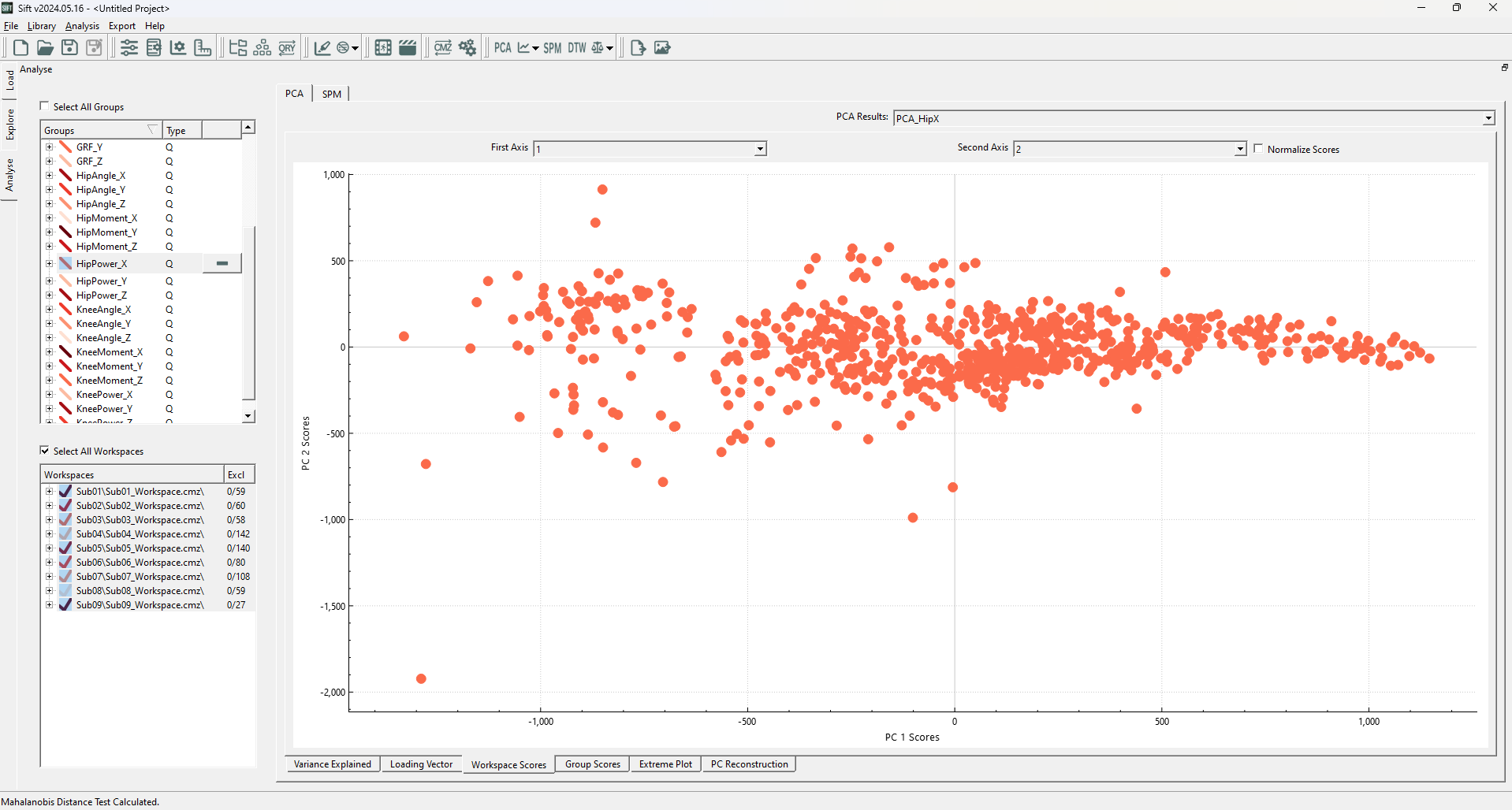
After calculating the PCA Results, the Workspace Scores on the analyse page should look as follows (note that the points are coloured by group. If they were coloured by workspace, you would see many of these clusters correspond to workspaces):

We can clearly see an issue with using Euclidean Distance: while the dimensions do not covary (as PCA creates an independent basis), the PC1 clearly has a larger variance that should be accounted for. We are interested in automatically and algorithmic-ally removing the outliers that don't follow our general observations, and will use the Mahalanobis Distance Test and SPE to do so. To do so, open the Outlier Detection Using PCA dropdown on the toolbar, and select “Mahalanobis Distance Test and SPE”.

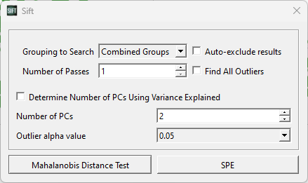
A pop-up window will appear, allowing you to customize some features for both test calculations. For this test, we should set the parameters as below (in the image):

For now, we are looking for outliers from within the entire PCA analysis. We could partition it such that points only calculate their LOF against points in their own group or workspace (which we will show later), but for now we want to look at the whole graph as one, and as such we have selected “Combined Groups”.

We choose to use 2 PCs, as the workspace scores are presented in 2 dimensions.

The Outlier alpha value is a tuneable parameter within the Mahalanobis Distance Calculation, which will determine the distance threshold for a data point to be classified as an inlier/outlier. The alpha value corresponds to the statistical significance of the chi-square distribution being compared to (i.e. a lower alpha value corresponds to a higher threshold needed to be an outlier, but more certainty in the results). Within SPE, the alpha parameter is similarly used, but corresponds to a non-central chi-square distribution instead.

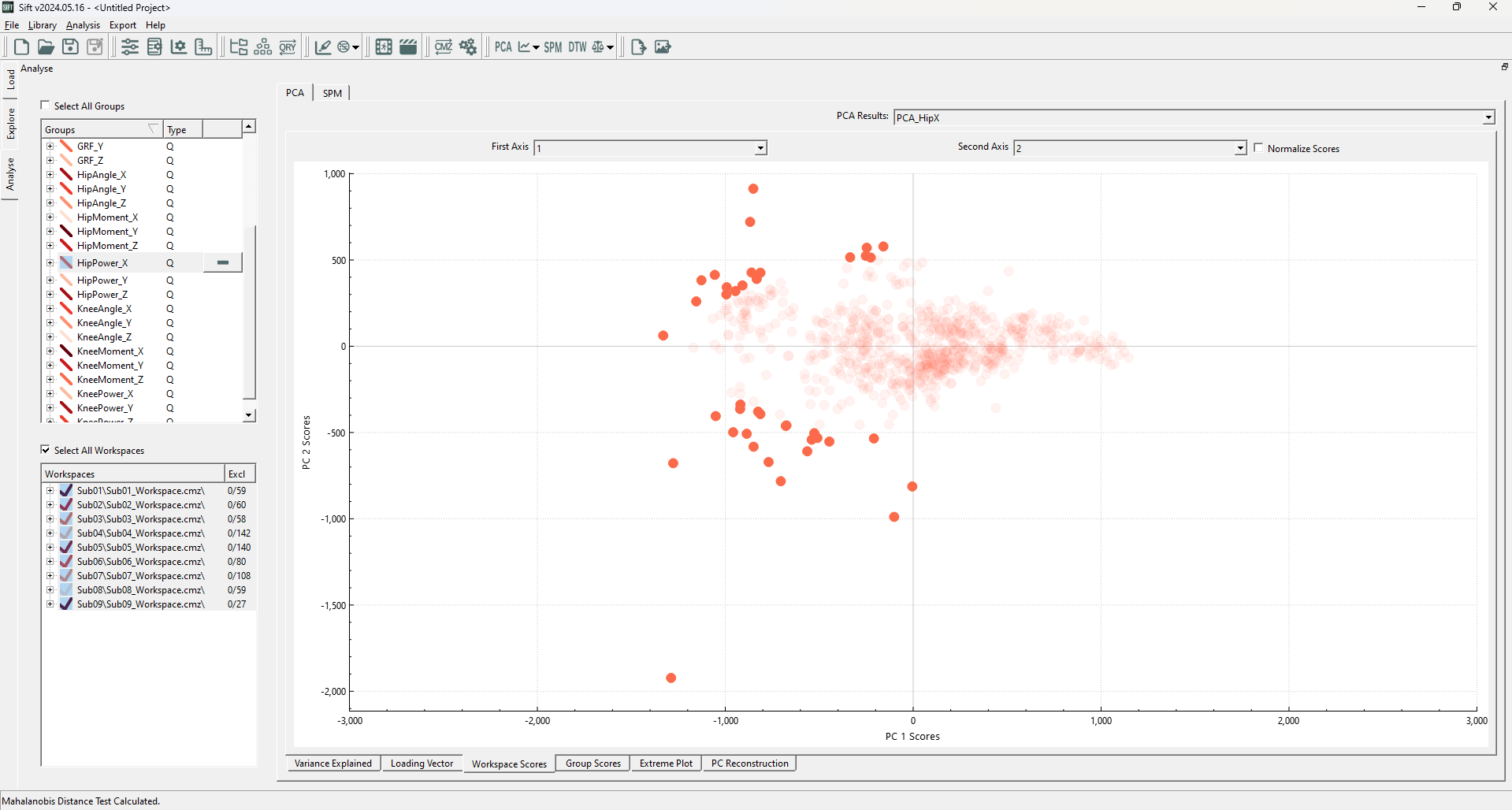
Upon running the Mahalanobis Distance Test, you should see the following datapoints highlighted (note that we rescaled the PC1 axis to have equivalent spacing to the PC2 axis):

We can immediately see that there are outliers whose (rough) Euclidean distance is much smaller than some of the inliers (ex: points near the PC1 axis at roughly +/-500 in the PC2 axis are closer than those along the PC2 axis at roughly +/-1000 in the PC1 axis). Using a normal distance measure would identify these differently, but because we used the Mahalanobis Distance Test, we were able to identify those that do not follow the general trend of the data.

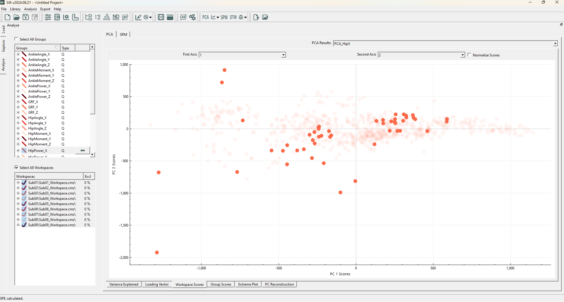
Upon running the SPE Test, you should see the following datapoints highlighted:

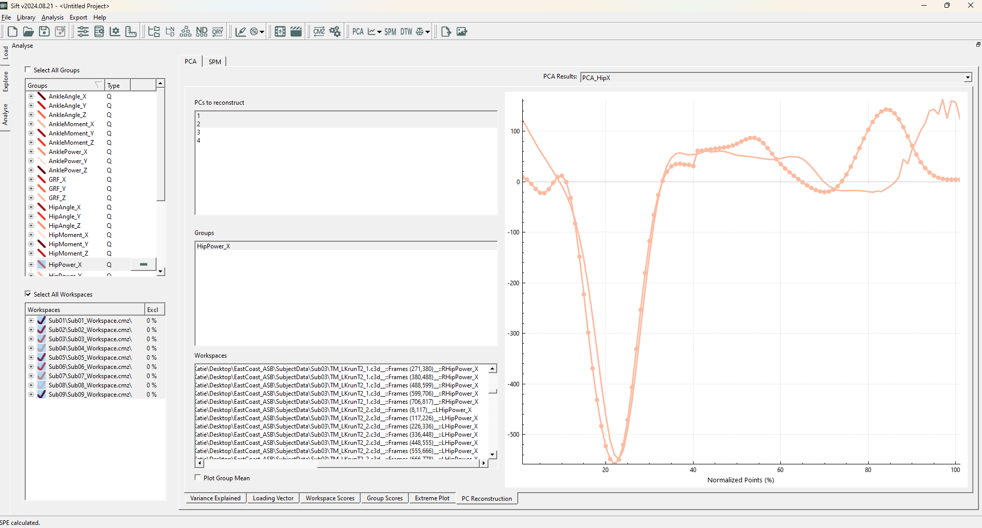
We notice that the outliers are seemingly random, some far away from the origin, while others are well within the 2D cluster. This is because SPE measures the reconstruction error! And not error within the lower dimensional representation. We can clearly see this through the PC Reconstruction page, if we plot one of the identified outliers (Sub04::OG_LA_run01.c3d::Frames(419,529)):

We can see there are some very clear errors in comparison to the ground truth! If you plot an inlier, you would see significantly less errors in this projection.