Table of Contents
Foot and Ankle Angles
Joint Angles are conceptually challenging to present concisely and accurately.
A joint angle is the relative orientation of one segment relative to another segment, and mathematically is often represented as a 3×3 rotation matrix.
The most common way to present the joint angle, however, is to parse this 3×3 rotation matrix into 3 components using an Euler sequence. The conceptual challenge is that there are 16 different Euler sequences by which this 3×3 rotation matrix can be parsed, and each sequence produces 3 different component values for a given 3×3 rotation matrix.
It seems intuitively clear that there must be a standard choice of the correct sequence for a given anatomical joint, but unfortunately, this is not the case.
Preparing for the Tutorial
1) Ensure that version 3.0 or later of Visual3D has been downloaded and installed.
2) Download the cmo file with the standing calibration file and model template from the website: Tutorial1.cmo
3) Launch the Visual3D program from the Start menu.
The program will open to the main workspace.
Purpose
1. Discuss the minimal marker placement for a single segment foot: Foot Segment - Marker Placement
2. Discuss the right-hand rule and its application to defining joint angles: Ankle Angle Explained
3. Create a simple foot definition which can be used for kinetic calculations: Kinetic Right Foot Segment
3. Use three different methods to define the foot for kinematic calculations:
Discussion
There are many ways to define the foot. With a simple single segment foot, two feet are often used:
1) The first foot is used for kinetic calculations, with the proximal joint is define at the ankle.
2) The second foot (often referred to as Virtual Foot) is used for kinematic calculations. The segment coordinate system of the kinematic foot is defined in such a way that the joint angle has a more clinically relevant meaning.
There is no set definition of neutral ankle angle, but neutral is approximately when the foot is flat on the floor and the shank segment is vertical. Since the angle joint and toe target are not parallel to the floor, an initial offset is introduced in the ankle angle. The segment coordinate system of the kinematic foot is defined to remove this initial offset and create a more clinically relevant ankle joint angle.
This tutorial will explain 3 ways to define a kinematic only foot. Keep in mind, there is no default Visual3D foot definition, and the correct definition is dependent on your laboratory's definition of neutral.
Note that although segments are defined using different proximal and distal landmarks, all segments are tracked using the same targets (RFT1, RFT2, RFT3). Also, since these feet are kinematic only, the radius is irrelevant and can be set to 0.1.
Foot Segment - Marker Placement
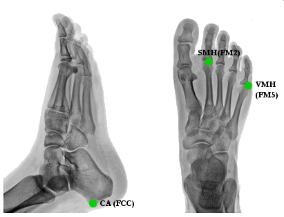
The placement of the calcaneous marker is then very important. The height of the calcaneous marker relative to the height of the toe marker defines dorsi-plantar flexion in the standing posture. Medial lateral placement of the calcaneous marker is important because the sagittal plane of the foot is defined by the calcaneous marker, the toe marker, and the virtual ankle center.
CA[1](FCC) [2]:p. 160 = Posterior Surface of Calcaneus
ST[1](FST)[2]:p. 160 = Sustentaculum Tali of Calcaneus
SMH[1](FM2)[2]:p. 160 = Head of 2nd Metatarsus
VMH[1](FM5)[2]:p. 160 = Head of 5th Metatarsus
VMB[1](FMT)[2]:p. 160 = Tuberosity of 5th Metatarsal
PM[1](PM6)[2]:p. 160 = Proximal Medial Phalanx
FMB[1] = Base of First Metatarsal
SMB[1] = Base of Second Metatarsal
- As previously mentioned, Visual3D does not have a default marker set or segment definition. It is therefore important to keep in mind that the marker set and segment definitions described in this tutorial as solely provided as an example. There are a number of alternatives for marker placement and segment definition.
Create a Kinetic Right Foot Segment
This is a simple representation of the foot that is adequate for many of the Kinematic and Kinetic calculations in Visual3D. It is not, however, adequate for the calculation of the ankle joint angle.
If using the Sample Data provided in the beginning of this tutorial, the Right Foot is defined in this way:
Virtual Foot Method 1 - Heel to Toe
This method will use the heel and toe targets to define the proximal and distal ends of the foot.
Creating the Ankle and Toe Joint Centers
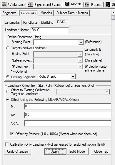
In this tutorial we consider the Ankle Joint Center to be the distal end of the shank segment:
Once the Ankle Joint Centers have been created, the Foot segments can now be defined.
Defining the Virtual Foot Segments
Note: This definition assumes that the heel, toe, and ankle center define the sagittal plane of the foot. Care must be taken to place the heel marker carefully. Any medial/lateral misplacement of the heel marker will result in an inappropriate inversion/eversion of the segment.
Rotating the Virtual Foot Segments
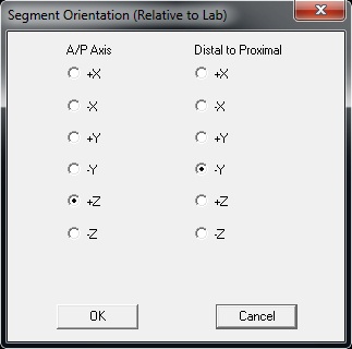
4. Rotate the Segment Coordinate System of the Right Virtual Foot Segment: The segment coordinate system should be rotated so the coordinate system follows the convention below: The x-Axis (red) represents flexion/extension of the ankle The y-Axis (green) represents inversion/eversion The z-Axis (blue) represents abduction/adducation Please see the Rotate Segment Coordinate System section of this tutorial for instructions on rotating the segment coordinate system. | 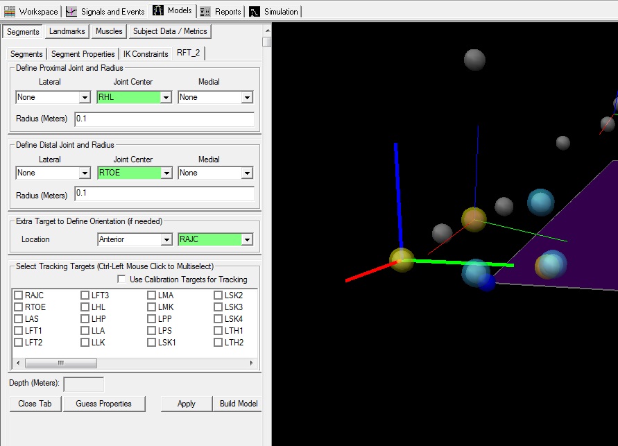 |
Virtual Foot Method 2 - Normalize to Proximal Segment
One method for setting the Ankle Joint Angle to Zero degrees in the standing trial is to define the Segment Coordinate System for the Virtual Foot Segment to be aligned precisely with the Segment Coordinate System for the Shank.
This can be accomplished by using the same proximal and distal targets.
Note: this definition assumes that the posture in the standing trial is to be considered an ankle angle of zero degrees regardless of the actual posture.
NOTE Since the two segment coordinate systems are perfectly aligned the segments have identical orientation in the standing trial and hence have a joint angle of zero degrees.
(The segment coordinate system in this section will not need to be rotated to follow the convention in the rest of the tutorial)
Virtual Foot Method 3 - Projected landmarks
Note: This definition assumes that the foot segment is parallel to the floor regardless of the actual posture in the standing trial.
Create 3 Laboratory Landmarks
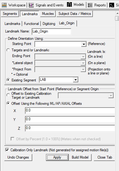
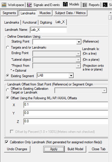
Create 3 landmarks (Lab_Origin, Lab_X, Lab_Y) to represent the lab.
Create 3 projected landmarks
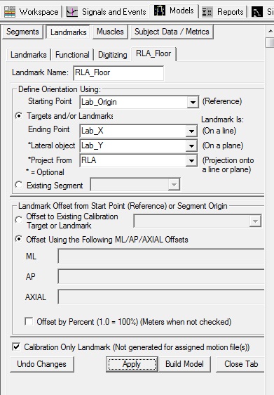
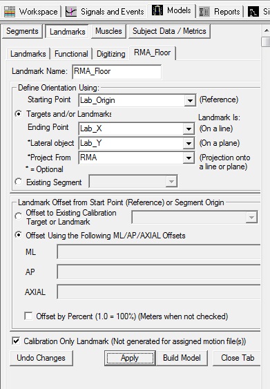
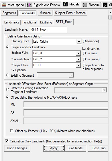
Create 3 landmarks (RLA_Floor, RMA_Floor, RFT1_Floor) that are the projection of the 3 markers used to define the foot onto the floor.
Create the Virtual Foot Segment
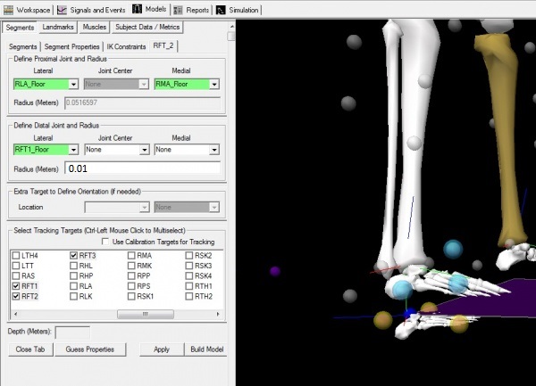
The following method creates a foot coordinate system that is aligned with the laboratory coordinate system (as established by the 3 landmarks created above). Since the landmarks are projected onto the floor, the Segment Coordinate System for the Virtual Foot will be parallel to the floor.
This orientation is convenient for describing the angle of the foot segment relative to a surface. In this example, the ankle joint angle will be close to zero in the standing posture (if the shank is vertical, the angle will be zero).
Rotate the Virtual Foot Segments
2. Rotate the Segment Coordinate System of the Right Virtual Foot Segment: The segment coordinate system should be rotated so the coordinate system follows the convention below: The x-axis (red) represents flexion/extension of the ankle The y-axis (green) represents inversion/eversion The z-axis (blue) represents abduction/adducation Please see the Rotate Segment Coordinate System section of this tutorial for instructions on rotating the segment coordinate system. |
Rotate Segment Coordinate System
Note that the segment coordinate system is parallel to the floor but the z-axis lies in the plane of the floor rather than vertical (e.g. aligned more-or-less with the shank coordinate system). To resolve this:
| Rotate the foot coordinate system: 1. In the Segment Properties tab, select Right Virtual Foot in the Segment Name box. 2. Click the Modify Segment Coordinate System button. | 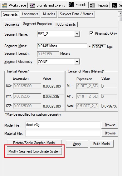 |
Ankle Joint Angle
A final example of this tutorial can be seen in this file.
Once this tutorial complete, a total of four foot segments have been defined:
Right Foot was defined using Kinetic Foot Segment
RFT_2 was defined using **Method 1** - Heel to Toe
RFT_3 was defined using **Method 2** - Normalized to proximal segment
RFT_4 was defined using **Method 3** - Projected Landmarks
The Ankle Joint Angle can be defined using the Virtual Foot relative the Shank segment. The joint angle created by each foot definition can be plotted and compared to see which is the most ideal definition for your specific task.
Ankle Angle Explained
Understanding the Ankle Angle Signal
This section will explain a little more about the definition of the ankle and the right hand rule.
The graphs in this section are saved in a cmo file which can be downloaded here.
Right Hand Rule
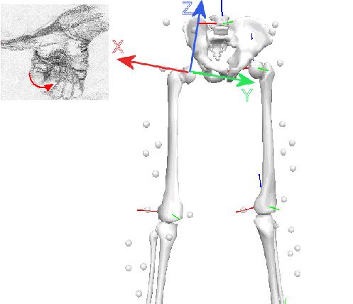 | For this segment coordinate system (z-up, y-anterior) rotation about the x-axis represents flexion/extension. Visual3D always computes all signals based on the Right Hand Rule. For example, if you point your thumb in the direction of the x-axis of the hip (shown in Red in the animation viewer) pointing laterally to the right. Knee extension will be zero when the thigh segment coordinate system and the shank segment coordinate system are aligned. Your curled fingers indicates the positive direction of rotation. Thus, in this case knee extension will be seen as a positive angle, and knee flexion as negative. Note that the x-axis for both the left and right thigh segment coordinate systems points laterally to the right. Using the same schema inversion of the ankle is a positive rotation about the y-axis for the right leg and a negative rotation about the y-axis for the left leg. Inward internal rotation of the ankle is a positive rotation about the z-axis for the right leg and negative rotation about the z-axis for the left leg. This reflection of the data anatomically from right to left is a result of applying the right hand rule rigidly within Visual3D. When presenting data it is quite common for Visual3D users to negate the y and z terms for the left knee angle so that the frontal and transverse plane rotation use the same sign convention for both right and left joint angles. |
Define the Ankle Angle (Following the Right Hand Rule for both sides)
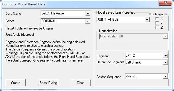
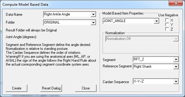
Define the Left and Right Ankle Angles in Compute Model Based:
1. Go to the Model drop down menu
2. Select Compute Model Based Data
3. Define the ankle angle using the following convention
NOTE: RFT_2 and LFT_2 are virtual feet which were created using **Method 3** in this tutorial.
Graph the Ankle Angle (without consistent sign convention)
Graph the X Y and Z components of the Ankle Angle:
The signals can be graphed as an interactive graph under the Signals and Events tab, or as a 2D graph under the Report Tab.
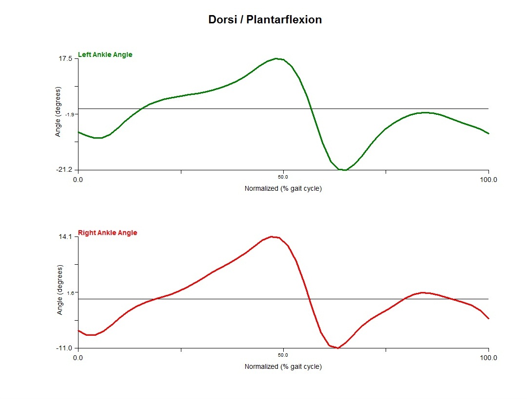 Left: + Dorsiflexion Right: + Dorsiflexion | 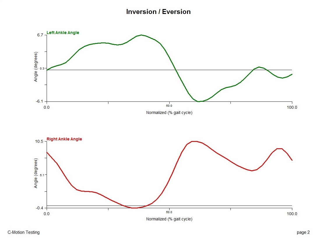 Left: + Eversion Right: + Inversion | 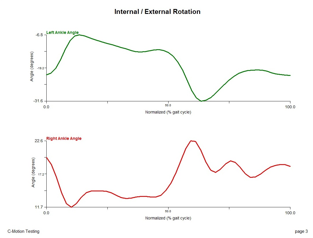 Left: + Abduction Right: + Adduction |
As per the above description, because the Right Hand Rule is being applied strictly followed for both right and left joint angles, the sign conventions are opposite between right and left side for the frontal and transverse plane. Though not a problem in itself, in biomechanics it is often recommended to use the same sign convention for both sides so that interpreting joint angles is easier.
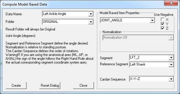
Define the Ankle Angle (Sign convention using the Right Hand Rule from the Right side only)
Define the Left and Right Ankle Angles in Compute Model Based:
Negating a component simply multiplies the signal by -1, to change its sign convention.
Graph the Ankle Angle (with consistent sign convention)
Graph the X Y and Z components of the Ankle Angle:
 Left: + Dorsiflexion Right: + Dorsiflexion | 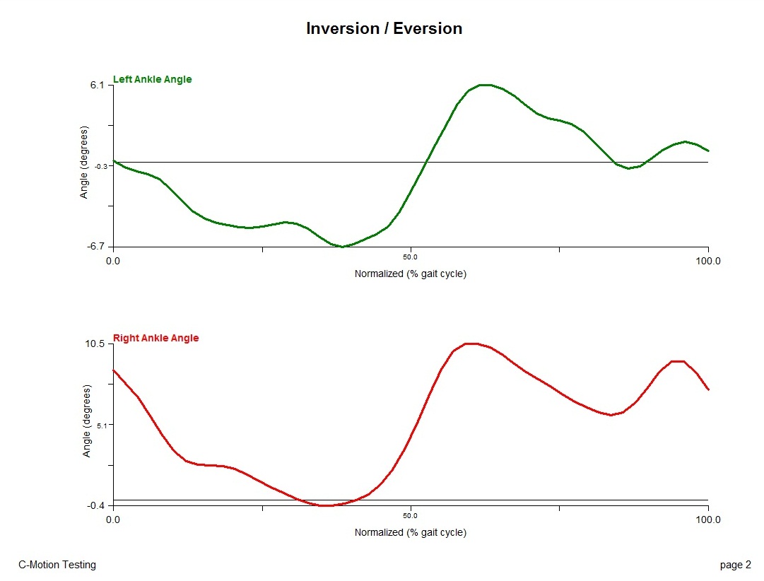 Left: + Inversion Right: + Inversion | 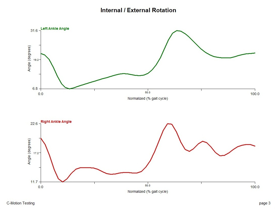 Left: + Adduction Right: + Adduction |
The resulting rotations about the y-axis/frontal plane (abd/adduction) are positive in the same direction.
The resulting rotations about the z-axis/transverse plane (internal/external rotation) are positive in the same direction.
Foot Progression Angle
The foot progression angle is a measure often used in clinical settings, to assess toe-in/toe-out during gait. While the exact way of computing the Foot Progression Angle can vary, this tutorial describes two of the most common ways.
Please note that neither of the proposed methods in this tutorial is the method used by Vicon in Nexus and referred as Foot Progression Angle.
Using a Virtual Lab
When using a model that includes a Pelvis segment, it is recommended to create a Virtual Laboratory that will change with the direction of walking. This allows to compute consistent Pelvic angle, without being affected by the direction of walking.
The same also applies to the Foot Progression Angle. To compute the progression angle relative to the lab, it is important that the reference coordinate system used is consistent with the direction of walking.
Create a Virtual Lab
First, create a Virtual Laboratory that changes with the direction of walking. Once completed, you can proceed to the next step to compute the foot progression angle.
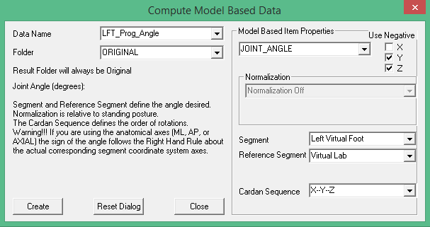
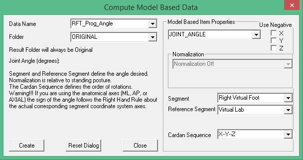
Define the Foot Progression Angle
Compute the Foot Progression Angle using Compute Model Based Data:
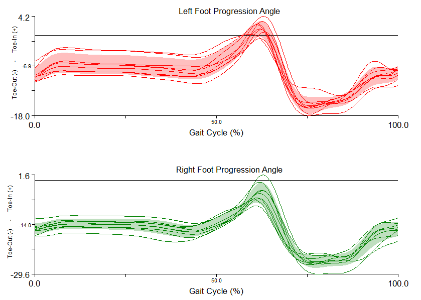
Graph the Foot Progression Angles
Considering that the Foot Progression Angle is a measure of Toe-In/Toe-Out, only the “Z” component of the L/RFT_Prog_Angle should be used and graphed:
Using the General Pelvis Direction
Another method to compute Foot Progression Angle is to use the general direction of the pelvis as the main direction of progression.
A vector is created using the position of the Pelvis' CG at the first and last frame of each trial, a second vector created using the long axis of the foot (i.e. running anterior-posterior). The angle between these two vector, projected onto the lab floor is then computed, for both the left and the right foot.
Pipeline Script
This pipeline script is markerset dependent. The user will need to modify the marker names accordingly in order for it to work correctly. The changes should be made in the Evaluate_Expression, following the Compute right-side unit vector and Compute left-side unit vector comments. The markers are those of the “toe” and “heel”, representing the center line of the foot.
Event_Explicit
/EVENT_NAME=START
/FRAME=1
! /TIME=
;
Event_Explicit
/EVENT_NAME=END
/FRAME=EOF
! /TIME=
;
!
! Find Pelvis at start
!
Metric_Signal_Value_At_Event
/RESULT_METRIC_NAME=Pelvis_At_START
! /RESULT_METRIC_FOLDER=PROCESSED
/SIGNAL_TYPES=KINETIC_KINEMATIC
/SIGNAL_NAMES=CGPOS
/SIGNAL_FOLDER=RPV
/EVENT_NAME=START
/GENERATE_MEAN_AND_STDDEV=FALSE
! /APPEND_TO_EXISTING_VALUES=FALSE
! /GENERATE_VECTOR_LENGTH_METRIC=FALSE
! /RETAIN_NO_DATA_VALUES=FALSE
;
!
! Find Pelvis at start
!
Metric_Signal_Value_At_Event
/RESULT_METRIC_NAME=Pelvis_At_END
! /RESULT_METRIC_FOLDER=PROCESSED
/SIGNAL_TYPES=KINETIC_KINEMATIC
/SIGNAL_NAMES=CGPOS
/SIGNAL_FOLDER=RPV
/EVENT_NAME=END
/GENERATE_MEAN_AND_STDDEV=FALSE
! /APPEND_TO_EXISTING_VALUES=FALSE
! /GENERATE_VECTOR_LENGTH_METRIC=FALSE
! /RETAIN_NO_DATA_VALUES=FALSE
;
!
! Convert metric signal by grabbing an arbitrary signal multiplied by zero and add metric
!
Evaluate_Expression
/EXPRESSION=0.0*KINETIC_KINEMATIC::RPV::CGPOS+METRIC::PROCESSED::Pelvis_At_END
/RESULT_NAME=Signal_Pelvis_At_END
! /RESULT_TYPE=DERIVED
! /RESULT_FOLDER=PROCESSED
;
!
! Convert metric signal by grabbing an arbitrary signal multiplied by zero and add metric
!
Evaluate_Expression
/EXPRESSION=0.0*KINETIC_KINEMATIC::RPV::CGPOS+METRIC::PROCESSED::Pelvis_At_START
/RESULT_NAME=Signal_Pelvis_At_START
! /RESULT_TYPE=DERIVED
! /RESULT_FOLDER=PROCESSED
;
Evaluate_Expression
/EXPRESSION=vector((DERIVED::PROCESSED::Signal_Pelvis_At_End::X-DERIVED::PROCESSED::Signal_Pelvis_At_START::X),
(DERIVED::PROCESSED::Signal_Pelvis_At_End::Y- DERIVED::PROCESSED::Signal_Pelvis_At_START::Y),
(0*(DERIVED::PROCESSED::Signal_Pelvis_At_End::Z-DERIVED::PROCESSED::Signal_Pelvis_At_START::Z)))
/RESULT_NAME=DirectionOfProgression
! /RESULT_TYPE=DERIVED
! /RESULT_FOLDER=PROCESSED
;
Signal_Magnitude
/SIGNAL_TYPES=DERIVED
/SIGNAL_NAMES=DirectionOfProgression
/SIGNAL_FOLDER=PROCESSED
/RESULT_NAMES=DirectionOfProgression_Magnitude
/RESULT_TYPES=DERIVED
/RESULT_FOLDER=PROCESSED
! /RESULT_SUFFIX=
;
Evaluate_Expression
/EXPRESSION=DERIVED::PROCESSED::DirectionOfProgression/DERIVED::PROCESSED::DirectionOfProgression_Magnitude
/RESULT_NAME=DirectionOfProgression_Unit
! /RESULT_TYPE=DERIVED
! /RESULT_FOLDER=PROCESSED
;
!
! Compute right-side unit vector
!
Evaluate_Expression
/EXPRESSION=vector((TARGET::PROCESSED::RTOE::X-TARGET::PROCESSED::RFCC::X),
(TARGET::PROCESSED::RTOE::Y-TARGET::PROCESSED::RFCC::Y),
(0.0*(TARGET::PROCESSED::RTOE::Z-TARGET::PROCESSED::RFCC::Z)))
/RESULT_NAME=RFoot_Line
! /RESULT_TYPE=DERIVED
! /RESULT_FOLDER=PROCESSED
;
Signal_Magnitude
/SIGNAL_TYPES=DERIVED
/SIGNAL_NAMES=RFoot_Line
/SIGNAL_FOLDER=PROCESSED
/RESULT_NAMES=RFoot_Line_Magnitude
/RESULT_TYPES=DERIVED
/RESULT_FOLDER=PROCESSED
! /RESULT_SUFFIX=
;
Evaluate_Expression
/EXPRESSION=DERIVED::PROCESSED::RFoot_Line/DERIVED::PROCESSED::RFoot_Line_Magnitude
/RESULT_NAME=RFoot_Line_Unit
! /RESULT_TYPE=DERIVED
! /RESULT_FOLDER=PROCESSED
;
!
! Compute left-side unit vector
!
Evaluate_Expression
/EXPRESSION=vector((TARGET::PROCESSED::LTOE::X-TARGET::PROCESSED::LFCC::X),
(TARGET::PROCESSED::LTOE::Y-TARGET::PROCESSED::LFCC::Y),
(0.0*(TARGET::PROCESSED::LTOE::Z-TARGET::PROCESSED::LFCC::Z)))
/RESULT_NAME=LFoot_Line
! /RESULT_TYPE=DERIVED
! /RESULT_FOLDER=PROCESSED
;
Signal_Magnitude
/SIGNAL_TYPES=DERIVED
/SIGNAL_NAMES=LFoot_Line
/SIGNAL_FOLDER=PROCESSED
/RESULT_NAMES=LFoot_Line_Magnitude
/RESULT_TYPES=DERIVED
/RESULT_FOLDER=PROCESSED
! /RESULT_SUFFIX=
;
Evaluate_Expression
/EXPRESSION=DERIVED::PROCESSED::LFoot_Line/DERIVED::PROCESSED::LFoot_Line_Magnitude
/RESULT_NAME=LFoot_Line_Unit
! /RESULT_TYPE=DERIVED
! /RESULT_FOLDER=PROCESSED
;
!
! Steps left is to find unit vector of two landmarks on the right virtual foot Y
!
Evaluate_Expression
/EXPRESSION=cross(DERIVED::PROCESSED::RFoot_Line_Unit, DERIVED::PROCESSED::DirectionOfProgression_Unit)
/RESULT_NAME=RFoot_Line_Cross_Product
! /RESULT_TYPE=DERIVED
! /RESULT_FOLDER=PROCESSED
;
Evaluate_Expression
/EXPRESSION=asin(DERIVED::PROCESSED::RFoot_Line_Cross_Product::Z)
/RESULT_NAME=RFoot_Angle
! /RESULT_TYPE=DERIVED
! /RESULT_FOLDER=PROCESSED
;
Multiply_Signals_By_Constant
/SIGNAL_TYPES=DERIVED
/SIGNAL_NAMES=RFoot_Angle
/SIGNAL_FOLDER=PROCESSED
! /RESULT_NAMES=
! /RESULT_TYPES=
! /RESULT_FOLDER=PROCESSED
/RESULT_SUFFIX=_Degrees
! /SIGNAL_COMPONENTS=
/CONSTANT=57.3
;
!
! Steps left is to find unit vector of two landmarks on the left virtual foot Y
!
Evaluate_Expression
/EXPRESSION=cross(DERIVED::PROCESSED::LFoot_Line_Unit, DERIVED::PROCESSED::DirectionOfProgression_Unit)
/RESULT_NAME=LFoot_Line_Cross_Product
! /RESULT_TYPE=DERIVED
! /RESULT_FOLDER=PROCESSED
;
Evaluate_Expression
/EXPRESSION=-1*asin(DERIVED::PROCESSED::LFoot_Line_Cross_Product::Z)
/RESULT_NAME=LFoot_Angle
! /RESULT_TYPE=DERIVED
! /RESULT_FOLDER=PROCESSED
;
Multiply_Signals_By_Constant
/SIGNAL_TYPES=DERIVED
/SIGNAL_NAMES=LFoot_Angle
/SIGNAL_FOLDER=PROCESSED
! /RESULT_NAMES=
! /RESULT_TYPES=
! /RESULT_FOLDER=PROCESSED
/RESULT_SUFFIX=_Degrees
! /SIGNAL_COMPONENTS=
/CONSTANT=57.3
;
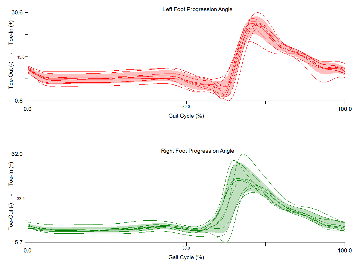
Graph the Foot Progression Angles
This method created a derived signal, make sure to select DERIVED in the Signal Type dropdown list, in the Y Axis Properties in the Add / Modify Graph window.

