Table of Contents
Using Statistical Parametric Mapping in Biomechanics
Statistical Parametric Mapping (SPM) is a method to create “Maps” of arbitrary statistical tests, which can be applied across the entirety of a continuous curve. These maps exist in the same dimensional space as their underlying data, which allows for the results to be more interpretable, as well as removing bias relating to selecting summary statistics like maximums, minimums or averages. Using random-field-theory, the inherent dependence between the parameters on these maps can be accounted for when determining how statistically relevant the results of a map are.
The Utility of SPM
Statistical tests, such as a T-Test, are useful tools used by scientists and statisticians, but they can fall prey to biases when trying to apply them to continuous data. At which point should these be applied? The maximum value? 50% through the gait cycle? All biomechanics signals have variance to them, and while registering these signals can help align them for better analysis, all the information outside of these specially chosen points will be lost, when it could be useful to our analysis. This is the key benefit to using SPM: continuous statistical inference in the original space of the data, allowing for more insights and intuitive understanding of the results.
The Math behind SPM
All of the math behind SPM is done internally with Sift, but we give a brief summary of it here for your purposes in Sift. Please refer to the references for more detailed explanations.
The GLM
The basis of SPM begins with modeling our data with a General Linear Model (GLM). A GLM is simply relating our data to an experimental design. This experimental design (in the form of a matrix) represents the experiment, and may represent what group or condition a trial belongs to (i.e. a 1 in the column that the trial belongs to, and 0 otherwise, etc.). We relate these though the formula:
Where Y is our original data, X represents out experimental design, B is a regression matrix (to be estimated using a Moore-Penrose inverse) and e is the resulting residuals.
This GLM allows us to apply arbitrary linear tests to each data point (i.e. a point in time for a gait analysis), such as a t-test or ANOVA, creating a “Statistical Parametric Map”, existing in the same n-dimensional space as the original data points (ex. 101 time data points for a normalized gait cycle).
T-Tests
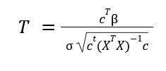
For a t-test, we model the GLM as above, with the design matrix consisting of 1's indicating a grouping for each test, and 0's otherwise. The SPM is evaluated with:
where c is a contrast vector indicating how we are selecting from our regression matrix (B), ^T represents a transposed matrix, sigma is the square-root of our variance, and X is our design matrix. The calculation for sigma is shown below:
where diag() is the diagonal values in a vector, e is the residuals, I represents the number of trials we have modeled (the # of rows in our Y Matrix), and rank(X) is equal to the number of groups (for a t-test, this would be 2).
This equation for T follows a T-distribution of degrees of freedom equal to I - rank(X).
ANOVA
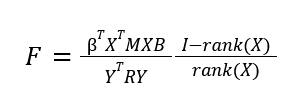
For our ANOVA tests, we model the GLM slightly differently. Instead of the design matrix including just the groupings, we add an additional term to represent the group-level effect (i.e. effect of all groups together), which is represented by all 1's in the design matrix. This is because the ANOVA test requires a “full” model (with group-level and individual group effect included), and a “reduced” model(with just the group-level effect modelled), which it compares. The contrast is applied slightly differently as well: we use it to help us form the full model and reduced models, using a projection matrix.
Where B is the ANOVA regression matrix, X is the design matrix, M is our projection matrix, and R is the “residual forming matrix”, which is similar to the projection matrix, and is the matrix which when applied to Y returns the given residuals.
The SPM follows a F-distribution with degrees of freedom rank(X) and I - rank(X).
Random Field Theory
With n samples in our map, it would be sound to estimate the significance with a Bonferroni correction, but we know that spatially similar data points in biomechanics are intrinsically dependent on each other, and thus the Bonferroni assumption of independence between data points would result in a far more conservative than necessary significance. As such, Random Field Theory (rft) is employed to estimate the dependence between data points (called smoothness), and to establish a threshold for statistical significance of the data. This can be represented with the familiar p-values for simple t-tests.
Which test to use
Choosing your experimental hypothesis is very important, and this should influence the statistical test being undertaken. ANOVA provides us a broad look at all of our data: with the hypothesis that all groups have the same mean, we can easily test IF there is 1 or more groups not following this hypothesis, but we cannot discern which one it is. T-tests on the other hand can specifically tell us if any 2 groups are different, and specifically identify which tests are different.
For many groups, it is recommended to first use an ANOVA test, and if there is statistical differences, to use post-hoc t-tests with a bonferroni correction (or the Holm–Bonferroni method) to identify which group this is.
For related groups, it is recommended to use a paired t-test over a two-sample t-test, as it has strictly higher statistical power.
Visualizing SPM Results
Visualizing your SPM results is important, and is broken down in the SPM Analyse Page.
This page includes:
- Visualizing the maps;
- Visualizing the statistics;
Tutorials
For a step-by-step example of how to use Sift to perform SPM on your data, and to interpret the results, see the SPM Tutorial.
Reference
Our implementation of Statistical Parametric Mapping is based articles by Todd Pataky, as well as the ___ textbook on the topic: “Statistical Parametric Mapping - The Analysis of Functional Brain Images”:
K. Friston, J. Ashburner, S. Kiebel, T. Nichols, and W. Penny, Statistical Parametric Mapping: The Analysis of Functional Brain Images, 1st ed.; Academic Press: Cambridge, MA, USA, 2006; ISBN 978-0-08-046650-7.
Description
In an age where the amount of data collected from brain imaging is increasing constantly, it is of critical importance to analyse those data within an accepted framework to ensure proper integration and comparison of the information collected. This book describes the ideas and procedures that underlie the analysis of signals produced by the brain. The aim is to understand how the brain works, in terms of its functional architecture and dynamics. This book provides the background and methodology for the analysis of all types of brain imaging data, from functional magnetic resonance imaging to magnetoencephalography. Critically, Statistical Parametric Mapping provides a widely accepted conceptual framework which allows treatment of all these different modalities. This rests on an understanding of the brain's functional anatomy and the way that measured signals are caused experimentally. The book takes the reader from the basic concepts underlying the analysis of neuroimaging data to cutting edge approaches that would be difficult to find in any other source. Critically, the material is presented in an incremental way so that the reader can understand the precedents for each new development. This book will be particularly useful to neuroscientists engaged in any form of brain mapping; who have to contend with the real-world problems of data analysis and understanding the techniques they are using. It is primarily a scientific treatment and a didactic introduction to the analysis of brain imaging data. It can be used as both a textbook for students and scientists starting to use the techniques, as well as a reference for practicing neuroscientists. The book also serves as a companion to the software packages that have been developed for brain imaging data analysis.
Pataky TC (2010) Generalized n-dimensional biomechanical field analysis using statistical parametric mapping. Journal of Biomechanics 43. 1976-82 ([1])
Abstract
A variety of biomechanical data are sampled from smooth n-dimensional spatiotemporal fields. These data are usually analyzed discretely, by extracting summary metrics from particular points or regions in the continuum. It has been shown that, in certain situations, such schemes can compromise the spatiotemporal integrity of the original fields. An alternative methodology called statistical parametric mapping (SPM), designed specifically for continuous field analysis, constructs statistical images that lie in the original, biomechanically meaningful sampling space. The current paper demonstrates how SPM can be used to analyze both experimental and simulated biomechanical field data of arbitrary spatiotemporal dimensionality. Firstly, 0-, 1-, 2-, and 3-dimensional spatiotemporal datasets derived from a pedobarographic experiment were analyzed using a common linear model to emphasize that SPM procedures are (practically) identical irrespective of the data's physical dimensionality. Secondly two probabilistic finite element simulation studies were conducted, examining heel pad stress and femoral strain fields, respectively, to demonstrate how SPM can be used to probe the significance of field-wide simulation results in the presence of uncontrollable or induced modeling uncertainty. Results were biomechanically intuitive and suggest that SPM may be suitable for a wide variety of mechanical field applications. SPM's main theoretical advantage is that it avoids problems associated with a priori assumptions regarding the spatiotemporal foci of field signals. SPM's main practical advantage is that a unified framework, encapsulated by a single linear equation, affords comprehensive statistical analyses of smooth scalar fields in arbitrarily bounded n-dimensional spaces.


