X4D Overview

X4D tracks 3D objects (bones, implants, etc.) in X-ray images by generating digitally reconstructed radiographs (DRRs) of the objects and matching them to the X-ray images. It requires that the 3D X-ray configuration parameters be defined in the subject file and that the X-ray images be corrected.

To match DRR images to X-ray images, both sets of images are processed first. X-ray images are smoothed with a convolution filter, and then an edge detection algorithm is performed on them. The final processed X-ray image that is used for tracking is the edge detection image times a weighting factor, plus the smoothed intensity image. DRR images are not smoothed, but are input to the edge detection algorithm. The final processed DRR image is the edge detection image time a weighting factor, plus the original DRR image.

Bone Tracking

4D Optimization

4D optimization tracks one or more objects by solving all frames in the tracking range at the same time. It works using a simulated annealing optimization process over two passes. In the first pass, a temporary pose map is created by evaluating the object’s pose map over the tracking range at equal time stamps. The object poses at these times are the control points that the optimizer varies to find the global solution. The spacing between the time stamps is determined by the Frame Spacing (Pass 1) parameter. For example, if the parameter is set to 4 and there are 20 reporting times in the tracking range, there will be 20 / 4 + 1 = 6 poses in the pose map-- a pose at each end of the range and 4 poses equally spaced between them. The algorithm then proceeds to optimize each control point independently of the others, while evaluating the DRR/X-ray matching for the X-ray frames in the neighborhood of the control point. The size of this neighborhood is determined by the Frame Envelope (Pass 1) parameter. For example, if the parameter is set to 2, each time the optimizer changes the pose at one of the time stamps, it will evaluate the DRR/X-ray matching at the closest X-ray frame to that time (in each view), and in the 2 frames on either side of that closest frame. In the second pass, a temporary pose map is created by evaluating the optimized pose map from the first pass at equal time stamps. This process is the same as described above, but uses the Frame Spacing (Pass 2) parameter to determine the spacing. The algorithm then optimizes each control point independently, evaluating a neighborhood of frames determined by the Frame Envelope (Pass 2) parameter. For this second pass, the number of simulated annealing iterations per control point is halved, the translation and rotation ranges are divided by four, and the initial temperature is divided by four. Once the second pass is complete, its final pose map is evaluated at the reporting times in the tracking range and those poses are inserted into the object’s pose map.

Matching Xray and DRR Images

The process of matching the DRR images to the X-ray images is sensitive to the image processing parameters in the X-ray/DRR Settings widget. Once the DRR images have been generated for a particular set of bone poses the DRR images and the X-ray images are processed (using an identical method) and then compared to each other. The algorithm used to compare them, called the image metric, can be selected in the Object Tracking widget. The processing method consists of: performing a Sobel edge detection on the image, thresholding the edge-detection image (which is controlled by the Edge Capping values in the X-ray and DRR Settings widget), multiplying the edge-detection image by a weighting factor (which is controlled by the Edge/Intensity Merge value in the X-ray and DRR Settings widget) and adding it to the original image, thresholding the merged image, and scaling the result. Pixels in the edge image whose values are greater than the Edge Capping maximum are set to zero. Very bright pixels (sharp edges) are usually inorganic objects like EMG electrodes or metal plates or wires. They can be removed from the edge image by lowering the Edge Capping maximum from 100. Every pixel in the edge image whose value is above the Edge Capping minimum is set to the Edge Capping minimum. This effectively strengthens weaker edges (those below the Edge Capping minimum) because the entire image is scaled later. For example, if the Edge Capping values are set to 5 and 30, every pixel in the edge image that is greater than 30 is set to 0. Every pixel that is between 5 and 30 is set to 5. The resulting edge image has all pixels between 0 and 5, with many of the edges of interest set to 5, making them all equally strong. After the edge image has been weighted and added to the original image, the result is thresholded using the Image Threshold values. All pixels above the Image Threshold maximum are set to the maximum, and all pixels below the Image Threshold minimum are set to 0. Much of the time these thresholds should be left at 100 and 0. However, there are times when it is useful to raise the minimum above zero to mask soft tissue regions, and lower the maximum from 100 to remove artificial edges, such as the end of a CT bone that is within the X-ray image. Note: the Image Scale Value is used in step 5. The final processed image is scaled linearly so that all pixels are in the range 0 to this scale value. Most of the time the scale values for the X-ray and DRR images should both be set to 255.0, but occasionally there are times when it is helpful to scale one image more than the other (e.g., when most of the bone edges in a DRR image are too dull because of one bright area that scales to 255.0). The success of the bone tracking algorithm is particularly sensitive to the Edge Capping minimum for the X-ray images. A change in this value of 2 or 3 (percent) can make a big difference in the solution found by the optimization. If you find that the optimization is locking into a bad pose with the edge capping minimum set to 10, try lowering the minimum to 7 or 8 (or even 5) and trying again. When you start processing a new data set, it can take some trial and error to figure out the set of image processing parameters that produce the best results. It is recommended that you start by tracking the bones (individually) in a single frame, trying different parameter values until the optimization algorithm can lock onto the correct pose for each bone. Then try solving a few adjacent frames to see if the same parameter values work on those.

Motion Capture Data

Working with Motion Capture Data

If you have surface-marker-based motion capture data for an x-ray trial, you can use it to calculate initial poses for the bones you want to track in the trial. To use this data in X4D, you must have C3D files with labelled marker trajectories for the motion trial and its associated static trial, and Visual3D files defining a kinematic model and its motion constraints. In the DSX software, this model is referred to as a mocap model. Creating the model template and the constraint scripts requires a good working knowledge of Visual3D. The model template file (MDH) defines the segments and landmarks in the kinematic model, based on a specific marker set. The build script (V3S) creates the constraints that define the relative motions of the segments in the model. The recalc script (V3S) updates the segment poses to satisfy the constraints. Once the model is defined, and applied to a particular DSX trial, it can be used in three modes: Marker Mode - The motions of the segments are driven by the surface markers, with constraints enforced. This mode is used to calculate mocap poses in X4D. Interactive Mode - You can interactively change all of the model's degrees of freedom (the 6 degrees of freedom of the root segment, and the joint angles). Constraints are enforced. This mode is used when you manipulate the bone poses in X4D. DSX Mode - The motions of the segments are driven by DSX tracking results (transform matrices). Constraints are not enforced. This mode is used when DSX results are viewed and analyzed in Visual3D. In addition to generating initial poses for the tracking objects, you can use the mocap model to help with manual positioning of the objects. In the Mocap Model widget in X4D, you can turn on the model's joint constraints, making it easier to move all of the objects together as a group, or to move them relative to each other in a realistic manner (e.g., flexing or twisting the vertebrae in a spine model).

Menus

File Menu

The Load Subject command loads a Subject file. This command can also be accessed with the Ctrl + O shortcut.       The Save Subject command saves the currently loaded subject to its existing Subject file. This command can also be accessed with the Ctrl + S shortcut.       The Save Subject As command saves the currently loaded subject to a new Subject file.       The Load Pose Maps command loads an existing pose map file for each selected object. You will be prompted to browse for each file, which must be saved as a .csv file.       The Save Pose Maps command saves the pose map of each selected object in the current trial to a .csv file. This file contains 6 values for each pose: the XYZ translation and the XYZ Euler angles representing the transform from the xray lab frame to the object's local coordinate system (i.e., as if you were traveling from the lab frame to the object frame). If a name for the pose map file is not already specified in the subject file, you will be prompted to browse for the file to create. A link to this file will then be added to the subject file.       The Save Pose Maps As command saves the pose map for each selected object in the current trial to a new .csv file. You will be prompted to browse for a new file for each object. A link to this new file will then be added to the Subject file.       The Save Object Transforms command saves the pose map of each selected object in the current trial to a .txt file. This file contains a 4x4 transform for each pose, expressing the transform from the xray lab frame to the object's local coordinate system (i.e., as if you were traveling from the lab frame to the object frame). If a name for the transforms file is not already specified in the subject file, you will be prompted to browse for the file to create. A link to this file will then be added to the subject file.       The Save Landmarks command saves the locations in the xray lab frame of each selected object's landmarks in the current trial. This file contains a set of landmark coordinates for each pose in the pose map. If a name for the landmarks file is not already specified in the subject file, you will be prompted to browse for the file to create. A link to this file will then be added to the subject file.       The Export Poses to CMZ command exports the pose map of each selected object in the current trial to the session's CMZ file. This requires that the CMZ already contain a C3D file for the current trial, with a kinematic model that includes segments for the selected objects.       The Exit command exits the program and all unsaved data will be lost. The program can also be closed by using the X in the top right corner of the program window.

View Menu

The view menu controls which screen widgets are displayed       The Body Reference Frames control toggles the display of the local coordinate systems of the selected objects in the xray windows and the 3D view. It can also be toggled using Alt + R.       The Body Landmarks control toggles the display of the landmarks of the selected objects in the xray windows and the 3D view. It can also be toggled using Alt + L.       The DSX Configuration control toggles the appearance of the dockable DSX Configuration widget. It can also be controlled using the Ctrl + Shift + C shortcut.       The 3D View control toggles the appearance of the dockable 3D View window. It can also be controlled using the Ctrl + Shift + V shortcut.       The Output control toggles the appearance of the dockable Output window. It can also be controlled using the Ctrl + Shift + O shortcut.       The Xray/DRR Settings control toggles the appearance of the dockable Xray/DRR Settings widget. It can also be controlled using the Ctrl + Shift + X shortcut.       The Pose Maps control toggles the appearance of the dockable Pose Maps widget. It can also be controlled using the Ctrl + Shift + A shortcut.       The Object Tracking control toggles the appearance of the dockable Object Tracking widget. It can also be controlled using the Ctrl + Shift + T shortcut.       The Image Optimization control toggles the appearance of the dockable Image Optimization widget. It can also be controlled using the Ctrl + Shift + I shortcut.       The Graphs control toggles the appearance of the dockable Graphs widget. It can also be controlled using the Ctrl + Shift + G shortcut.       The Mocap Model control toggles the appearance of the dockable Mocap Model widget. It can also be controlled using the Ctrl + Shift + M shortcut.

Options Menu

CPU Threading With two CUDA-capable graphics cards, object tracking speed can be increased when each of these cards is controlled by its own CPU thread. To assist with customer support, C-Motion staff might occasionally ask to disable CPU threading.      X-Ray Opacity The opacity of the X-ray images in the 2D and 3D windows. Their opacity should be less than 1.0 so that the DRRs can be seen superimposed on them. The default value is 0.5.      Simulated Annealing Temp The initial temperature for the ASA simulated annealing algorithm. The higher the initial temperature, the more slowly the search range will narrow during the optimization. The default value is 2000.      Color Theme The user can choose between a light and dark color theme.       When more than one CUDA-capable graphic cards are installed in the computer, the Select Gpus command opens a modal dialog that allows you to select the graphics card to be used for each view. Currently only one gpu per view is supported. The Alt-G shortcut can also be used to open this dialog. The menu item is disabled when there are none or just one CUDA-capable graphic card installed.

Help Menu

The Help command opens the X4D wiki page in the default browser. The F1 shortcut can also be used.       The System Information command opens a dialog with information about your computer, including available RAM and graphics card specifications.       The About option displays a dialog with information about X4D, including the installed version number. It also contains the Deactivate button, for deactivating your DSX suite license.

Widgets

DSX Configuration

Subject The Subject field is automatically populated with the ID of the subject when you load a Subject file.      Session The Session drop down menu is automatically populated with all of the sessions available available for the current subject.      Configuration The Configuration drop down menu is automatically populated with all of the configurations available for the current session.      Trial The Trial drop down menu is automatically populated with all of the trials available for the current configuration.      Object The Object list is automatically populated with all of the objects in the current trial. Each object is enabled if it is trackable, meaning that it has a 3D image file associated with it, for generating DRRs.

X-ray and DRR Settings

The matching of DRR images to X-ray images is sensitive to the image processing parameters in this widget. Once the DRR images have been generated for a particular set of bone poses, the DRR images and the X-ray images are processed (using an identical method), and then compared to each other using the selected image metric algorithm. The processing method consists of performing a Sobel edge detection on the image, thresholding the edge-detection image multiplying the edge-detection image by a weighting factor and adding it to the original image, thresholding the merged image, and scaling the result. The parameters that control this process are in the X-ray/DRR Settings widget. Their descriptions can be found here.

Pose Maps

A pose map is the set of poses for a tracked object. Each pose expresses the transform from the X-ray (lab) frame to the object’s anatomical frame (i.e., as if you were traveling from the lab frame to the object frame), and is at one of the trial’s reporting times. Each of the 6 DOFs in a pose map is interpolated (and possibly smoothed) with a GCV (generalized cross-validation) spline. Smoothing of pose map splines is controlled by the Pose Map Cutoff Frequency parameter. Pose maps are stored in CSV files.      Add Current Poses to Maps For each selected object, add its pose at the current reporting time to its pose map.      Clear Current Poses From Maps For each selected object, removes from its pose map the pose at the current reporting time.      Clear Pose Maps Clears all poses from the pose maps of the selected objects.      Smooth Pose Maps For each selected object, replaces each pose in the pose map with one calculated by evaluating the splines at the pose time. Note: the resulting splines may still not pass through the smoothed poses because of the nature of GCV cut-off frequency smoothing.

Object Tracking

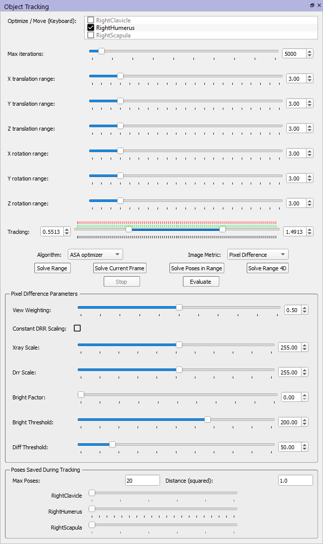
Optimize These check boxes let you specify which objects are allowed to move during the tracking optimization. DRRs for all of the objects selected in the Object Configuration panel will be generated, but only the objects selected here will be allowed to move. This allows you to perform hierarchical tracking, such as tracking the femur, then fixing it in its optimized pose while tracking the patella.      Max Iterations The maximum number of iterations for one pass of the optimization algorithm. For single-frame optimization, this is the number of iterations for one frame (reporting time). For 4D optimization, this is the number of iterations for the first pass. For the second pass of 4D, half of this number is used as the maximum.      Translation Ranges There is a slider for each of the X, Y, and Z translation ranges. Each one controls the amount that the DOF is allowed to change from its initial value during optimization.      Rotation Ranges There is a slider for each of the X, Y, and Z rotation ranges. Each one controls the amount that the DOF is allowed to change from its initial value during optimization.      Tracking The range of reporting times which will be optimized when using the Solve Range, Solve Poses in Range, or Solve Range 4D commands.      Solve Range Starts the frame-by-frame optimization process. The selected objects’ poses are optimized at each reporting time in the tracking range. It starts at the current time and proceeds towards the earliest, then goes back to the current time and proceeds towards the latest. Although each frame (reporting time) is optimized independently of the others, previously optimized frames will modify the pose map, which could affect the starting poses for subsequent frames. Note: the optimization will execute much faster if you turn off the display of the DRRs and CT objects in the 2D and 3D windows.      Solve Current Frame Performs an optimization of the current frame. Note: the optimization will execute much faster if you turn off the display of the DRRs and CT objects in the 2D and 3D windows.      Solve Poses in Range Performs an optimization of each reporting time in the tracking range that already has a pose specified in the pose map. Note: the optimization will execute much faster if you turn off the display of the DRRs and CT objects in the 2D and 3D windows.      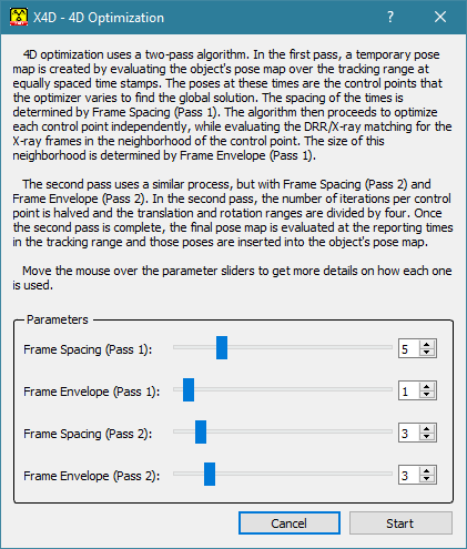Solve Range 4D Starts the 4D optimization process. The entire tracking range is optimized at the same time. Note: the optimization will execute faster if you turn off the display of the DRRs and CT objects in the 2D and 3D windows.      Frame Spacing (Pass 1) The interval of the reporting times when generating the pose map for the first pass of the 4D optimization algorithm. For the optimization, a pose map is created by evaluating the object’s pose map at every Nth reporting time. The default value is 5.      Frame Envelope (Pass 1) The number of frames near the control point to evaluate during the first pass of 4D optimization. A value of 0 means to evaluate only the frame in each view that is closest to the control point. A value of 3 means to evaluate the closest frame plus the 3 closest frames on each side of the control point, for a total of seven. The default value is 1.      Frame Spacing (Pass 2) The interval of reporting times when generating the pose map for the second pass of the 4D optimization algorithm. For the optimization, a pose map is created by evaluating the pose map optimized in the first pass at every Nth reporting time. The default value is 3.      Frame Envelope (Pass 2) The number of frames near the control point to evaluate during the second pass of 4D optimization. A value of 0 means to evaluate only the frame in each view that is closest to the control point. A value of 3 means to evaluate the closest frame plus the 3 closest frames on each side of the control point, for a total of seven. The default value is 3.      Optimizer (ASA, SPAN, LBFGSB) The type of optimization algorithm to use. ASA (adaptive simulated annealing) is currently the only recommended algorithm. SPAN is another type of simulated annealing. LBFGSB is a bounded, least-squares algorithm (local optimizer).      Stop Stops the currently running optimization.      Evaluate Performs a detailed analysis of the DRR/X-ray matching for the current reporting time with the currently selected objects. A summary of the results is written to the Output window, and TIFF images of the X-rays, DRRs, and X-ray/DRR correlations are written to the folder containing the subject file. The correlation images are color-coded as follows: red = the DRR pixel is not bright (its value is less than Eval Bright Threshold) cyan = the DRR pixel is bright and "good" compared to the X-ray pixel (the difference is less than Eval Good Threshold) greenscale = bright DRR pixel value - X-ray pixel value, when DRR value > X-ray value yellowscale = X-ray pixel value - bright DRR pixel value, when X-ray value > DRR value      Image Metric The algorithm used to compare the X-ray and DRR images.      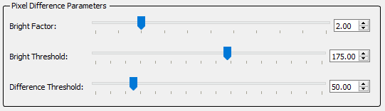Pixel Difference Each pixel in the processed DRR image is compared directly to its corresponding pixel in the X-ray image. To compare a DRR pixel to an X-ray pixel, first the absolute value of the difference between them is calculated. If this difference is greater than the Difference Threshold, and the DRR pixel value is greater than Bright Threshold, the difference is squared. This gives a greater weight to DRR pixels that are bright and which do not match well with their corresponding X-ray pixels. The pixel difference is then squared and multiplied by a brightness factor. This factor is 1.0 plus Bright Factor times the DRR pixel value. When Bright Factor is zero, bright DRR pixels are not weighted differently than any others. But when it is greater than zero, the DRR’s brightness is used to weight the error for that pixel. This is a second method of weighting a bright DRR pixel more heavily, without considering its difference with the X-ray pixel (as the first method does). The values for all pixels in each view are then summed to determine the fitness for that view. The sums for the two views are then multiplied to get the overall image correlation value, which the algorithm tries to minimize.      Conditional Entropy The cross-conditional entropy, H, of the DRR image relative to the X-ray image is calculated and minimized by the optimization algorithm. 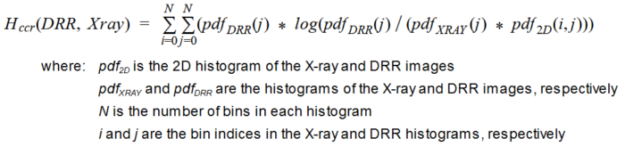Reference: Wang F, Vemuri B, Rao M, Chen Y (2003). Cumulative residual entropy, a new measure of information & its application to image alignment. Proceedings of the Ninth IEEE International Conference on Computer Vision, October, 2003. DOI: 10.1109/ICCV.2003.1238395.      Global Parameters These parameters, which are independent of the image metric algorithms, are used when comparing the X-ray images to the DRR images.      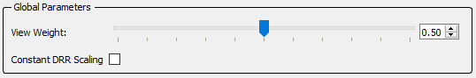View Weight This specifies the relative weight of the two views in the final image metric calculation (0.0 = all view 1, 1.0 = all view 2). The default value is 0.5, which means to weight each view equally. If you are tracking objects in single-plane image data (i.e., both views contain the same images), set this parameter to either 0.0 or 1.0 so that X4D will generate and evaluate DRRs for only one view, making the optimization twice as fast.      Constant DRR Scaling This boolean controls whether or not to scale the DRRs for each view by a constant value for all iterations of an optimization. If false, each DRR will be scaled so that its maximum value is equal to the DRR image scale value in the X-ray/DRR Settings widget. If true, a single scale value will be calculated during the first iteration and be used to scale the DRRs in all subsequent iterations.      Poses Saved During Tracking Sometimes the global minimum of the image fitness function is not the correct pose of the bone being tracked. This is often because the X-ray and DRR image processing parameters are not ideal (see Image Optimization, below). Other times, it is because the bone in the X-ray images is occluded by soft tissue or other bones, or because of inherent differences between X-ray images and DRRs (image resolution, X-ray scatter, CT thresholding, etc.). To account for these other times, the ASA tracking algorithm attempts to save bone poses that result in local minima of the cost function, while still searching for the global minimum. The idea is that if the correct bone pose is not the global minimum, it is likely to be a local minimum somewhere within the search range. The ASA algorithm thus attempts to save a set of local-minimum poses so that you can revisit them once optimization has finished. The Max Poses field specifies how many local minima to save. When the tracking optimization has finished, if the final bone pose is not the correct pose, you can re-apply the saved poses by dragging the slider for that bone. If one of them is correct (or at least better than the final pose), you can use the Add Current Poses to Maps command in the Pose Map widget to add that pose to the map, thus overwriting the final pose. Note: When the ASA algorithm evaluates a particular bone pose during optimization, it cannot determine if it is actually a local minimum or not because it does not compute gradients. It estimates if the pose is a local minimum by examining its cost function value and its proximity to other poses with similar values. Here is an example that details the process. If you perform an ASA optimization of 1000 iterations, with Max Poses set to 20 and Distance (squared) set to 3.0, when the optimization is complete the 1000 bone poses that were evaluated are sorted from lowest to highest cost function value. The pose with the lowest value is marked as the global minimum and added to the list of saved poses. Then the pose with the next lowest value is checked to see how close it is to the first pose. The sum of the squares of the differences in the 6 DOF values is computed and compared to the Distance (squared) value (3.0 in this case). If the distance is less than 3.0, it is assumed that this pose is in the same valley of the solution space as the first pose, so it should not be saved as a local minimum. If it is greater than 3.0, the pose is added to the saved pose list. Then the next pose in the sorted list is checked. If it is not within 3.0 units of any pose already in the saved list, it is added to the saved list. This process proceeds until the saved list contains 20 poses. It will take some trial and error to determine the best value of the Distance (squared) parameter for a particular data set, but a value in the range of 1.0 to 3.0 is reasonable, as the solution spaces are often very bumpy with numerous local minima. The units for the DOF translations are model units (usually mm), and the units for the rotations are degrees.

Image Optimization

Accurate tracking of bones is sensitive to the X-ray and DRR image processing parameters. In some cases it can take a significant amount of trial and error to determine the parameter values that enable the image matching algorithm to "lock in" on the correct bone pose. That is, the parameter values that cause the global minimum of the image fitness function to be at the correct bone pose. There are 15 different parameters, and sometimes changes of 1 or 2% in one of them can change the "optimal" bone pose by a few degrees or millimeters. The Image Optimization widget is a tool for automatically finding optimal values of the parameters. The sliders allow you to specify ranges for each of the 15 parameters in the Xray/DRR Settings widget, and the Max Iterations slider at the top is for specifying how many tracking optimizations to perform with randomly chosen parameter values within the specified ranges. Each tracking optimization proceeds as if you had selected Solve Current Frame in the Object Tracking widget. It optimizes the selected bones, starting at their current poses, and compares the final poses to the initial ones. The smaller this difference, the better the result. Please see How To: Optimize Xray/DRR Settings for a step-by-step guide on using this widget.

Graphs

In the Graphs widget you can display and edit the pose map of one of the selected objects. The graphs show the 6 DOFs of the object's pose at each reporting time. To display the graphs, select an object from the combo box in the upper left corner of the widget. With the checkboxes at the top you can individually control the display of the X, Y, and Z translations and the X, Y, and Z rotations (Euler angles). You can also select the type of spline used to interpolate the poses (GCV or linear), and the cutoff frequency used to smooth the GCV splines. The circles on the graphs represent the poses in the object’s pose map. The dashed lines are splines (GCV or linear) fit to the circles (control points) and smoothed with the cutoff frequency specified at the top. The gray region behind the curves represents the tracking range specified in the Object Tracking widget. The vertical green line shows the current reporting time. The graphs can be moved left, right, up, and down in the window using the Shift key and the left mouse button. The Y axis can be zoomed in and out using the mouse wheel. Pressing 'r' resets the graph axes to display the splines for all of the selected curves in that graph. Pressing Ctrl + 'r' resets the graph axes to display all of the control points of the selected curves. To move a control point, left-click on it and drag it up or down to a new location (you cannot change the time of a control point). You can select multiple points by pressing Ctrl while left-clicking on the points, or by sweeping a region while pressing the left mouse button. You can then move all selected points together by left-clicking on any of them and dragging up or down. To unselect all control points, left-click away from all points or press Esc. Note: moving control points in the graphs directly modifies the pose map that is loaded into X4D, and there is no undo feature. It does not, however, modify the pose map file; this can only be done by selecting Save Pose Maps from the File menu. Also, whenever a pose map is modified by any method in X4D, it is saved to a backup file in the same folder as the original pose map file.

Mocap Model

Time Offset The offset between the start of the x-ray data capture and the surface-marker motion capture. It is specified as the x-ray start time minus the motion capture start time.      Calculate Mocap Poses, Fixed Body, Mocap Seed Spacing If Fixed Body is set to none, then Calculate Mocap Poses will clear the pose maps for the objects selected in the Configuration widget and create new poses based on the motion capture data. Poses are created for the entire trial, using the value of the Mocap Seed Spacing parameter. For example, if the spacing is 5, then a motion capture pose will be calculated for every 5th reporting time in the trial. If Fixed Body is set to one of the tracked objects in the trial, then that object's pose map will not be modified by Calculate Mocap Poses. Instead, the pose maps for the other selected objects will be cleared. Then for each pose in the fixed object's pose map, the poses of the other objects will be calculated such that they satisfy the joint constraints relative to the fixed object and the generalized coordinates of the motion capture data. Note: One strategy for tracking multiple bones in a trial is to first Calculate Mocap Poses with no fixed body. This will position all of the bones using the surface markers in the motion capture data. Then track one of the bones for all frames in which it is trackable, deleting the extra mocap-based poses when you are done. Then Calculate Mocap Poses again, with Fixed Body set to the bone that you just tracked. The other bones will "snap into place" relative to the tracked bone. In other words, it will use the motion capture data to pose all the bones, then move them as a group so that the fixed bone lines up with its tracked pose.      Apply Joint Constraints When this option is selected, the constraints in the kinematic model specified for the trial are applied to the tracking objects. When you select it, the root object remains in its current pose, and the other objects are moved so as to satisfy the kinematic constraints. You can then move the entire model as a rigid unit by selecting and moving any object in it, and you can move the joints of the model by moving the generalized coordinate sliders below the checkbox.

3D View

The 3D View window displays a 3D scene representing the X-ray configurations and the tracking objects. The surface models generated from CT data can be manipulated by the user. To do so the model first needs to be selected by left-clicking on it. A trackball consisting of three circles and three lines will be displayed centered in and aligned with the selected object’s local (anatomical) coordinate system. The trackball allows the selected object to be manipulated as follows: 3D View When the left mouse button is depressed on one of the circles, the circle will be highlighted to visually indicate it is selected and when the mouse cursor is dragged across the screen (the left mouse button is still depressed), the object is rotated in the plane of the selected circle. When the left mouse button is depressed on one of the lines, the line will be highlighted to visually indicate it is selected and when the mouse cursor is dragged across the screen (the left mouse button is still depressed), the object is translated along the selected line. Left-clicking within the trackball without selecting any of the circles or lines, will highlight all circles. When the mouse cursor is dragged across the screen (the left mouse button is still depressed), freehand rotation of the object will occur. Left-clicking within the trackball without selecting any of the circles or lines but with depressing the shift key, will highlight all lines. When the mouse cursor is dragged across the screen (the left mouse button is still depressed), freehand translation of the object will occur. Left-clicking outside the trackball will make the trackball disappear and deselect the object. Note: moving an object this way does not move the other objects with it, even if Apply Joint Constraints is turned on.      Show Lab Toggles the display of the X-ray source, X-ray image frame, and projection line.      Show CT Toggles the display of the CT bones of the selected objects.      Show View 1 Image Toggles the display of the X-ray + DRR image for view 1.      Show View 2 Image Toggles the display of the X-ray + DRR image for view 2.      Show Axes Toggles the display of the X-ray lab reference frame.      Show Mocap Markers Toggles the display of the motion capture markers for the current reporting time.      Align View with X-Axis Moves the camera to look down the negative X axis.      Align View with Y-Asix Moves the camera to look down the negative Y axis.      Align View with Z-Axis Moves the camera to look down the negative Z axis.      Align View with View 1 Source Moves the camera to the x-ray source in View 1, and points it along the x-ray projection line.      Align View with View 2 Source Moves the camera to the x-ray source in View 2, and points it along the x-ray projection line.      Context Menu Context menu for 3D view Pressing the right mouse button will display a context menu with some of the functionality described above.

Xray Windows

The Xray windows display the xrays of each view, as well as the DRRs of all selected objects.      Moving the DRRs To move an object in one of the 2D xray windows, Shift-middle-click on the DRR to pick it. A reference frame will be displayed over it, with its origin at the center of the object's CT volume. To translate the object, Shift-left-click on the DRR and drag it to a new location. To rotate the object about the origin of the displayed reference frame, Ctrl-left-click on the DRR and drag the cursor. To unpick the object, press the Escape key or Shift-middle-click in the window away from any of the DRRs. Note 1: Moving objects with the mouse does not modify their pose maps. To save the new poses you must press the Add Current Poses to Maps button in the Pose Map widget. If you do not save the poses, they will be lost when you change the current reporting time. Note 2: If Apply Joint Constraints is turned on in the Mocap Model widget, all of the objects in the trial will move with the one you manipulate directly, even if they are not selected.      Mouse and Keyboard Commands The following mouse and keyboard commands are available in the 2D windows for interacting with the xray images and DRRs. The commands that move the objects move all objects selected in the DSX Configuration widget, whether or not they have been picked for interaction (with Shift-middle-click). To rotate all selected objects by +0.5 degrees about their local X, Y, and Z axes, press Ctrl and the X, Y, or Z keys. To rotate all selected objects by -0.5 degrees about their local X, Y, and Z axes, press Alt + Ctrl and the X, Y, or Z keys. To translate all selected objects by +0.5 mm along their local X, Y, and Z axes, press Shift and the X, Y, or Z keys. To translate all selected objects by -0.5 mm along their local X, Y, and Z axes, press Alt + Shift and the X, Y, or Z keys. The left, right, up, and down arrow keys translate all selected objects by 0.5 mm in the plane of the xray window. Pg Up/Down: moves to the previous/next reporting time. Home/End: moves to the first/last reporting time. ‘<’ and ‘>’ rotates the selected objects about an axis perpendicular to the screen. The mouse wheel zooms the xray image in and out. Press and hold the left mouse button to change the image contrast (move cursor left/right) and brightness (move cursor up/down). Press and hold the middle mouse button to pan the xray image within the window. H toggles the display of on-screen help text. C moves the selected objects in front of the X-ray images. R resets the position of the xray image in the window, as well as the brightness and contrast. S toggles the display of the xray image (same as Show Xray checkbox) D toggles the displays of the DRRs (same as Show DRR checkbox) P toggles whether the displayed xray is the raw image or the processed image (same as Show Processed Xray checkbox) O toggles whether the displayed DRRs are the raw ones or the processed ones (same as Show Processed DRR checkbox) Alt+R toggles the display of the selected objects' local coordinate systems Alt+L toggles the display of the selected objects' landmarks Note 1: Moving objects with keyboard commands does not modify their pose maps. To save the new poses you must press the Add Current Poses to Maps button in the Pose Map widget. If you do not save the poses, they will be lost when you change the current reporting time. Note 2: If Apply Joint Constraints is turned on in the Mocap Model widget, all of the objects in the trial will move with the one you manipulate directly, even if they are not selected.      Context Menu Context menu for 2D view Pressing the right mouse button will display a context menu with the following functionality (shortcut key between brackets): Select Drr: selects the drr under the cursor for manipulation. Show Xray (S): toggles the display of the xray image. Show Processed Xray (P): toggles whether the displayed xray is the raw image or the processed image. Show DRR (D): toggles the displays of the DRRs. Show Processed DRR (O): toggles whether the displayed DRRs are the raw ones or the processed ones. Move to First Frame (Home): moves to the first reporting time. Move to Previous frame (PgDown): moves to the previous reporting time. Move to Next Frame (PgUp): moves to the next reporting time. Move to Last Frame (End): moves to the last reporting time. Reset View (R): resets the position of the xray image in the window. Center Objects (C): moves the selected objects in front of the X-ray images. Toggle Help (H): toggles the display of on-screen help text.

Output Window
Shows progress and results of optimizations. Also shows results of image evaluation.