Global Optimization

In Visual3D the Inverse Kinematics problem is solved as a global optimization problem, which computes the pose of a model that best matches the mocap data in terms of a global criterion.

In other words global optimization is the search of an optimal pose of a multi-link model for each data frame such that the overall differences between the measured and model-determined marker coordinates are minimized in a least squares sense, throughout all the body segments. It considers measurement error distributions in the system and provides an error compensation mechanism between body segments, which can be regarded as a global optimization at the system level.

Our initial solutions to this problem were based on the following article:

Lu TW and O'Connor JJ (1999) Bone position estimation from skin marker coordinates using global optimization with joint constraints.
J Biomech 32: 129-134

Consider a point attached to a segment, whose location is represented by a vector in the Segment Coordinate System (SCS).

The location of the same marker is represented by vector in the Laboratory Coordinate System (LCS)

is computed by Visual3D model builder

is the 3D motion capture data recorded

The relationship between and is given by:

                      (1)

where:

is a rotation matrix from SCS to LCS, and

is the translation between SCS and LCS.

If a segment moves, the new orientation matrix and translation vector may be computed at any instant, given that at least three non collinear points are assumed stationary in the SCS (predetermined for a specific subject) and are recorded.

For the 6 DOF analysis described elsewhere, the rotation matrix and origin vector are computed at each frame of motion capture data by minimizing the sum of squares error expression:

          (2)

Equation 2 represents a constrained maximum-minimum problem that Visual3D solves using the method of Lagrangian multipliers (adapted from Spoor & Veldpaus, 1980).

Lu & O’Connor (1999) described a global optimization process where joint constraints added to the model can minimize the effect of sensor noise and soft tissue artifact. Lu and O’Connor termed this process Global Optimization. Visual3D uses the method of Global Optimization described by Lu and O'Connor, but we and others in the biomechanics community prefer the term Inverse Kinematics (IK). Inverse Kinematics is an extension to the 6 DOF pose estimation because if a joint is ascribed 6 degrees of freedom, the solutions are equivalent.

Figure A model comprised of a series of rigid segments connected by joints.

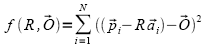
The solution to the IK is the pose of a model that best matches the motion capture data in terms of a global criterion (e.g. Least Squares). In the general case there is no analytic solution for the IK problem. Global optimization is the search of an optimal pose of a multi-link model such that the overall differences between the measured and model-estimated marker coordinates are minimized in a least squares sense at a system level. In the Lu and O-Connor approach the global optimization solution is found for each frame of data independent of any prior and later frames of data. Mathematically van den Bogert and Su (2008) described this approach based on the configuration of the total body based on a set of generalized coordinates. In this case, and of equation (1) become a function of all the generalized coordinates.

                (1)

Determining the observability from a set of data is an important concept for the IK.

Visual3D has 3 implementations of the solution to this optimization problem; in order of computational efficiency Levenberg-Marquardt, Quasi-Newton, and Simulated Annealing. Of particular relevance to this project is our implementation of the Quasi-Newton algorithm because this is a more stable method that we would prefer to use than the Levenberg-Marquardt algorithm, but is unfortunately slow to converge. (The Simulated Annealing algorithm is currently so slow that it is rarely used)

The Quasi-Newton algorithm is based on Newton's method for optimizing twice differentiable functions (Andrew, 2008). To understand Newton's method consider the function that starts at an initial point , moves through a series of points, and converges to a solution. Newton's method is a three step process: 1) compute the search direction, 2) determine the length of the next step and 3) use the results of steps 1 and 2 to obtain the new point. These steps are repeated until a local minimum is found.

To find the search direction (step 1) using Newton's method, consider a point on/near the current value. At, can be approximated by a 2nd order Taylor series expansion:

(5)

Where is the gradient ofat the current valueandis the Hessian or matrix of second partial derivatives at. Taking the gradient of this function we obtain:

The gradient has a minima at:

and thus the search directioncan be obtained from:

After solving for the search directionthe next point in the searchcan be found by moving in the direction ofwith a step size computed to ensure that we obtained a sufficient decrease in the cost function without taking excessively small steps. Onceis obtained it is checked against a termination criteria; if the criteria is met then the minima for the global IK problem is found, if the criteria is not met the process is repeated starting at step 1 withacting as the new current value

One problem with the Newton approach is that it requires computing the inverse of the Hessian matrixat each step. The Quasi-Newton method circumvents this problem by approximating the Hessian based on the changes in the gradient. In addition, Visual3D computes the gradientnumerically because it is difficult to obtain the explicit form of the gradient unless the hierarchical model is defined in an appropriate way. The result is that Visual3D has a very flexible, but slow IK method for estimating the pose.

In the Visual3D IK, each frame of data is computed "independently" of any other frame of data. The initial guess for the optimization algorithm at any given frame, however, is the state of the model at the previous frame. This may pose a problem because the solution at the previous frame might be an inappropriate local minima. The result is that pose estimates will diverge from the real solution by being stuck in this local minima. A common situation is that the subject enters the motion capture volume during the data collection. The first frame of complete data is often relatively unreliable, so the chances of getting trapped in a local minimum increase. A potential improvement to the algorithm is to compute the solution both forwards and backwards, in the hopes that one of the passes will land along a better solution path.

In many circumstances the IK solution is preferred to the 6 DOF solution, but the user must attend to the determination of the appropriateness of the joint constraints. For example, an experiment focused on understanding the kinematics of a damaged knee (e.g. Anterior Cruciate Ligament damage), might not benefit from an IK solution if the prescribed motion of the knee joint "hides" the pathology.

When estimating the pose the user may want to make sure that certain segments follow the tracking targets with a higher degree of accuracy than other segments. For example, the user may want the distance between the foot and the floor (or force platform) to remain similar to the values that would be obtained using a 6 DOF method. This can be accomplished by adding weight factors to the objective function:

(6)

where N is the number of generalized coordinates in the IK model andis the weight factor for each marker. In a similar vein, some sensors will not be considered representative of the pose because they are noisy, so the weight of these data can be reduced. The selection of the weights can be made pragmatically (heuristically) or rules may be used that allow the computation of an optimal set of weights.

It is well known that residual errors (i.e. differences between model predictions and sensor measurements) computed by IK algorithms reflect both sensor noise and soft tissue artifact. If these individual residuals are represented in their local segment coordinate system it is possible to compute correlations between the residuals and the generalized coordinates. What we really want to do is to identify systematic noise and minimize its effect on the estimated pose. The IK algorithm, however, has no mechanism to compensate for noise even though it can be used to identify the presence of systematic noise.

van den Bogert AT and Su A (2008) A weighted least squares method for inverse dynamic analysis. Computer Methods in Biomechanics and Biomedical Engineering, 11:1,3-9