Sift - Outlier Detection

Outlier Detection is encompassed in a variety of statistical methods which look to find data that is not representative of dataset to which it belongs. These outliers (or anomalies) may then be further analyzed, or simply discarded. There are a variety of different methods to do this, including supervised and unsupervised methods. Here we will describe some common detection methods, all of which have been implemented into Sift. Specifically, these methods are used to detect outliers using PCA Workspace Scores, the scores obtained by applying the PCA Loading vectors onto the original waveforms. This is computationally much cheaper than using original waveforms, as we use PCA to significantly reduce the dimensionality of the data, while retaining much of the variance. More information about PCA can be found on the PCA page.

Unsupervised Methods

Local Outlier Factor

Local Outlier Factor (LOF) is an unsupervised method of finding outliers through a data points local density, introduced in 2000 by Breunig et al. [[1]]. It compares the local density of each point to its local neighbours, and calculates a Local Outlier Factor as the average ratio between its own density and the neighbours. By doing so, it can find local outliers that a global method might not find.

The points o1 and o2 in the picture above both represent outliers. Some algorithms may not classify o2 as an outlier, as it has a similar density to the points in C1, but we see that based on the local tendencies of the data, it should be classified as an outlier.

The LOF is a statistic calculated for each point in the database, with values below 1 representing inliers (as they are in a denser neighbourhood than their k neighbours), while outliers are determined based on a threshold above 1, which should be tuned depending on the data being used. For more information on the implementation and guidelines for using this method, see the LOF section of our PCA Outlier Detection Tutorial.

Algorithm

1. Calculate the k-nearest neighbours:

   Using a distance metric (such as Euclidean Distance), calculate the k nearest neighbours for all data points.

2. Calculate reachability distance:

   For each point, calculate the reachability distance between itself and its k neighbours, defined as the maximum of:

   1. The distance between the 2 points.
   2. The distance from the neighbouring point to its own k-th nearest neighbour (known as the k-distance of the neighbouring point)

   Note that the use of reachability distance helps to normalize or smooth the output, by reducing the effects of random fluctuations (i.e. random points that are extremely close together)

   The reachability distance from p1 to o, and p2 to o is shown below:

   

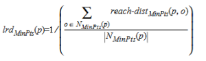
3. Calculate local reachability density:

   For each point, the local reachability density is 1 / (the average reachability distance to the k nearest neighbours), i.e.:

   

4. Calculate local outlier factor:

   For each point, the local outlier factor is the average ratio between the points local reachability distance and each of the local reachability distance of the k nearest neighbours, i.e.

   

5. Threshold to find outliers:

   Identify a threshold for which to determine points are outliers. This threshold should be some point above 1 (as a LOF of > 1 represents lower density than its neighbours), and should be done as a case by case basis. An automated method to choose a threshold is to use an iterated one-sided Grubbs outlier test on the LOF values, to determine outliers with a significance level alpha.

Grubbs' Outlier Test

The Grubbs' Outlier test is a method of finding a univariate outlier in normally distributed data. The test statistic represents the largest deviation from the sample mean (in terms of the standard deviation), and is compared against a t-distribution representing the stated significance level. The statistic is calculated as follows (for a one sided-maximal value test):

The null hypothesis of no outliers is rejected (at significance level a) if (i.e. we identify the maximal value as an outlier):

If we successfully reject the null hypothesis, we remove the outlier from the data, and calculate the statistic again on the new data. We can continue this until no outliers are detected, or stop after X outliers have been identified (X being up to the user).

Mahalanobis Distance Test

The Mahalanobis distance is a distance measure between a point and a distribution, which accounts for the covariance between each dimension in the distribution, essentially measuring the distance accounting for dependencies between dimensions, and the total variance along each dimension. This can be useful for finding datapoints which are close to inlier data, but don't follow the general trend observed.

The outliers in the picture above have very different Euclidean Distance measures (9.22 and 2.83 respectively), but have roughly the same Mahalanobis Distance Measures (6.16 and 6.00 respectively), indicating that both would classified as outliers at roughly the same level of confidence.

The Mahalanobis Distance is a statistic calculated for each point in the database, with larger distances indicating a higher likelihood that a point is an outlier (with a confidence threshold dependent on the # of dimensions being tested). For more information on the implementation and guidelines for using this method, see the Mahalanobis Distance section of our PCA Outlier Detection Tutorial.

The Mahalanobis Distance can be thought of as Euclidean distance where the dimensions have been de-correlated and scaled to unit variance. In fact, the Mahalanobis distance is exactly equivalent to Euclidean Distance, after performing a Whitening transformation, and is calculated as follows:

Where X is the vector difference of the point from the distribution mean, and S^-1 is the inverse of the variance-covariance matrix of the distribution.

The square of the Mahalanobis Distance (d^2) follows a chi-square distribution, and as such we can use this as a test statistic: The Mahalanobis Distance Test.

We produce this statistic for each data point being observed, and choose the null hypothesis to be that this point was drawn from the specified multi-variate normal distribution. We can reject this null hypothesis (at significance level alpha) if (i.e. the point is an outlier):

Where X^2(chi^2) is the chi-square distribution with n dimensions, at significance level alpha.

If we successfully reject the null hypothesis, we remove the outlier from the data, and calculate the statistic again on until we have calculated it on each data point. We can recalculate the new covariance, and continue this until no outliers are detected, or stop after X iterations have occurred (X being up to the user).

Squared Prediction Error (SPE)

SPE is a distance measure between the true measurement of a datapoint, and the predicted measurement of the datapoint. Unlike Mahalanobis Distance, this does not account for any of the variance in each dimension, but the total actual Euclidean distance. This is useful for finding data that is spatially far from a predicted value, even if it is well within a specified trend.

The example above shows an extended version of the Mahalanobis Distance example from above (in 3 dimensions), with a new datapoint

In the context of a PCA analysis, the SPE is a measurement of the PCA reconstruction error (i.e. how far off a PCA reconstruction from a lower dimensional space is from the original data). This is equivalent to the distance (squared) from the original data, to it's projection onto the PCA reduced k-dimension hyperplane, and is calculated as follows:

Where.....

The SPE is a direct

Reference

Markus M. Breunig, Hans-Peter Kriegel, Raymond T. Ng, and Jörg Sander. 2000. LOF: identifying density-based local outliers. SIGMOD Rec. 29, 2 (June 2000), 93–104. https://doi.org/10.1145/335191.335388

Abstract

For many KDD applications, such as detecting criminal activities in E-commerce, finding the rare instances or the outliers, can be more interesting than finding the common patterns. Existing work in outlier detection regards being an outlier as a binary property. In this paper, we contend that for many scenarios, it is more meaningful to assign to each object a degree of being an outlier. This degree is called the local outlier factor (LOF) of an object. It is local in that the degree depends on how isolated the object is with respect to the surrounding neighborhood. We give a detailed formal analysis showing that LOF enjoys many desirable properties. Using real-world datasets, we demonstrate that LOF can be used to find outliers which appear to be meaningful, but can otherwise not be identified with existing approaches. Finally, a careful performance evaluation of our algorithm confirms we show that our approach of finding local outliers can be practical.