Tutorial: Gait Profile Score and Movement Analysis Profile Pipeline
| Language: | English • français • italiano • português • español |
|---|
Academic Background
Baker et al. published two papers defining the calculation and applications of the Gait Profile Score (GPS):
- Baker, R., McGinley, J.L., Schwartz, M.H., Beynon, S., Rozumalski, A., Graham, H.K., Tirosh, O. (2009). The gait profile score and movement analysis profile. Gait Posture, 30(3), 265–269.
- Baker, R., McGinley, J. L., Schwartz, M., Thomason, P., Rodda, J., & Graham, H. K. (2012). The minimal clinically important difference for the Gait Profile Score. Gait Posture, 35(4), 612-615.
This tutorial describes how to create a pipeline to compute the Gait Profile Score and Movement Analysis Profile as detailed in the papers published by Baker et al.
Relevant Links
Downloads
GPS Description and Conventions
The Gait Profile Score (GPS) is a clinical index that can be used to measure the overall deviation of gait data relative to normative data. It is composed of Gait Variable Scores (GVSs) calculated from 9 key kinematic gait variables, which can be presented as a Movement Analysis Profile (MAP).

These kinematic variables are:
- Knee Flexion/Extension
- Ankle Dorsiflexion/Plantarflexion
- Pelvic Tilt
- Pelvic Rotation
- Pelvic Obliquity
- Hip Flexion/Extension
- Hip Abduction/Adduction
- Hip Rotation
- Foot Progression
Each of these kinematic variables should be normalized to the gait cycle (as in above right image), and should be sampled every 2% of the gait cycle (such that each signal has 51 points).
The GPS score can be computed for the left and/or the right side. It can also be computed as a overall index for both sides.
Please note: Since the pelvic movement is not specific to a any side, the authors recommend only including it when computing the GPS for the left side (as a convention). This means that for the left side, a total of 9 variables are used to compute the GPS, instead of only 6 for the right side. The overall GPS for both sides would therefore include all 9 variables.
Equations
Although calculating the Gait Profile Score was explained in Baker et al's 2009 paper, the equations were not explicitly written. Their 2012 paper contains explicit written equations but due to some formatting errors these are incorrect. The GPS Equations and Descriptions PDF has the correct version of these equations, which are also described below:
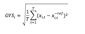
The Global Variable Scores (GVS) is the root mean square difference between a specific time normalized gait variable (x) and the mean data from the reference population calculated across the gait cycle (x ref).
|
i = the number of kinematic variables used t = the specific point in the gait cycle T = total number of points in the gait cycle xi,t = the value of gait variable i at point t xi,t ref = the mean of gait variable i at point t in the reference population If normalizing to every 2% of the gait cycle, T is equal to 51. |
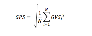
The Gait Profile Score (GPS) the root mean square average of all the Gait Variable Scores:
|
i = the specific kinematic variable T = total number of kinematic variables used If using 15 kinematic variables, N is equal to 15. |
As described in the previous section, the GPS can be calculated for the right side, the left side, or as an overall value. In Richard Baker's GPS Excel Sheet Calculator, there is also an added log transform to the final GPS value (this is optional).
Step 1: Model Creation and Joint Angle Definition
To calculate the GPS using the described kinematic variables, you must have a model with at least 7 segments:
- Pelvis
- Left/Right Thigh Segments
- Left/Right Shank Segments
- Left/Right Foot Segments
If you are unfamiliar with building models in Visual3D, the Model Building Tutorial is a good place to start if you want to alter the tutorial pipeline. The zip files for this tutorial contain a workspace with a pre-built and pre-applied model.
Once a model has been created, the joint angles for each of the nine kinematic variables need to be calculated. Below is an example of calculating the Left Ankle Angle:
!--------Left Ankle Angle----------!
Compute_Model_Based_Data
/RESULT_NAME=L_Ankle_Angle
/SUBJECT_TAG=ALL_SUBJECTS
/FUNCTION=JOINT_ANGLE
/SEGMENT=LMF
/REFERENCE_SEGMENT=LSK
/RESOLUTION_COORDINATE_SYSTEM=
! /USE_CARDAN_SEQUENCE=FALSE
! /NORMALIZATION=FALSE
! /NORMALIZATION_METHOD=
! /NORMALIZATION_METRIC=
! /NEGATEX=FALSE
! /NEGATEY=FALSE
! /NEGATEZ=FALSE
! /AXIS1=X
! /AXIS2=Y
! /AXIS3=Z
! /TREADMILL_DATA=FALSE
! /TREADMILL_DIRECTION=UNIT_VECTOR(0,1,0)
! /TREADMILL_SPEED=0.0
;
The zip file download for this tutorial contains a pipeline that calculates joint angles for all nine kinematic variables.
Step 2: Create a Normalized Database
To calculate GPS values a reference database needs to be created. The database should contain gait data with the same nine kinematic variables described above, which should be normalized to 51 points per gait cycle (in this tutorial, the gait cycles are defined as LHS to LHS).
The GPS_Tutorial_Files.zip contains a pre-made normalized database. The database uses the data from Subjects 2, 3 and 4. If you would like to create your own, the steps to do so can be found under the Normative Data from CMZ Library page. In Visual3D, databases are saved as .vnd file types.
Step 3: Calculating GPS Values using Visual3D Pipeline
This tutorial uses Subject 1 as the test subject and Subjects 2, 3 and 4 as reference subjects. Each subject has four exercises worth of data. The pipeline is approximately 1000 lines long, so it will be described rather than included in it's entirety on this page.
The GPS_Tutorial.zip contains two versions of this pipeline, one labeled "GPS_15features" which does not include the pelvis on the right side (as per Baker et als convention). This is the recommended pipeline to use. However, if you want to see the difference that including the pelvis on the right, there is also a pipeline labeled "GPS_18features".
- Calculating Joint Angles: For each of the kinematic variables (ankle angle, knee angle, hip angle, pelvis angle, foot progression) the Compute_Model_Based_Data command can be used to produce joint angle values. This is repeated once for the right side and once for the left side. The values are stored under the LINK_MODEL_BASED :: ORIGINAL folder.
- Create Global Signals for Joint Angles: The Global_Normalized_Mean function can be used to store specific components of a signal as a normalized global variable. In this case, the signals are normalized from LHS to LHS to 51 points, and we are interested in the following components of each kinematic variable, which are stored under the GLOBAL workspace in the P2D :: PROCESSED folder.
- Ankle Dorsiflexion: L_Ankle_Angle_X
- Knee Flexion: L_Knee_Angle_X
- Hip Flexion: L_Hip_Angle_X
- Hip Abduction: L_Hip_Angle_Y
- Hip Rotation: L_Hip_Angle_Z
- Pelvic Tilt: L_Pelvic_Angle_X
- Pelvic Rotation: L_Pelvic_Angle_Y
- Pelvic Obliquity: L_Pelvic_Angle_Z
- Foot Progression: L_Foot_Progression_Z
An example on how to normalize the left ankle to 51 points.
Global_Normalized_Signal_Mean
/SIGNAL_TYPES=LINK_MODEL_BASED
/SIGNAL_FOLDER=ORIGINAL
/SIGNAL_NAMES=L_Ankle_Angle
/SIGNAL_COMPONENTS=X
/COMPONENT_SEQUENCE=
! /START_LABEL=
! /END_LABEL=
/EVENT_SEQUENCE=LHS+LHS
! /EXCLUDE_EVENTS=
/RESULT_FOLDER=PROCESSED
/RESULT_NAME=L_Ankle_Angle_X
/NORMALIZE_POINTS=51
/CREATE_STANDARD_DEVIATION=TRUE
! /CALCULATE_PER_FILE=FALSE
;
Note: Step 3 and 4 are done in the Global Workspace
- 3. Open Reference Database: For the last two steps the normal database has to be loaded into the Visual3D workspace. This can be done using the File_Open command as seen below, however the file path will need to be changed on where you downloaded the normal database:
!------Open Normal Database------
! Note: file path may differ
File_Open
/FILE_NAME=C:\Users\amyco\Documents\GPS\GPS_Normalized_Database.vnd
! /SUFFIX=
!/SET_PROMPT=Open Control Database for GPS
;
- 4. Calculating GVS: For each axis of each joint, the reference signal is subtracted from the test signal, then the root mean square is calculated. This is repeated for right and left sides. Below is an example of calculating GVS for the right foot.
!--------Find GVS for Right Foot---------
Subtract_Signals
/SIGNAL_TYPES=P2D
/SIGNAL_NAMES=R_Foot_Progression_Z+R_Foot_Progression_Z_nd
/SIGNAL_FOLDER=PROCESSED
/RESULT_NAME=R_Foot_Progression_Z
/RESULT_FOLDER=R_GVS_Diff
;
Metric_Root_Mean_Squared
!Calculate the GVS
!The GVS is the RMS of the difference between the Subject and Control Data
/RESULT_METRIC_FOLDER=R_GVS
/RESULT_METRIC_NAME=_RMS
/APPLY_AS_SUFFIX_TO_SIGNAL_NAME=TRUE
/SIGNAL_TYPES=DERIVED
/SIGNAL_FOLDER=R_GVS_Diff
/SIGNAL_NAMES=R_Foot_Progression_Z
/COMPONENT_SEQUENCE=Y
/EVENT_SEQUENCE=
/EXCLUDE_EVENTS=
/SEQUENCE_PERCENT_START=
/SEQUENCE_PERCENT_END=
/GENERATE_MEAN_AND_STDDEV=FALSE
! /APPEND_TO_EXISTING_VALUES=FALSE
;
Evaluate_Expression
! Square the GVS value for each variable
/EXPRESSION=(METRIC::R_GVS::R_Foot_Progression_Z_RMS) ^ 2
!/SIGNAL_TYPES=METRIC
!/SIGNAL_FOLDER=R_GVS
! /SIGNAL_NAMES=
/RESULT_TYPES=METRIC
/RESULT_FOLDERS=R_GPS_MATH
/RESULT_NAME=R_Foot_Progression_RMS_SQR
! /APPLY_AS_SUFFIX_TO_SIGNAL_NAME=FALSE
;
- 5. Calculating GPS: The Evaluate_Expression function is used to implement the equation described above. The results are stored in the individual exercise files under the METRIC :: GPS folder. Below is an example of calculating the overall GPS.
!--------Calculate GPS----------
Add_Signals
/SIGNAL_TYPES=METRIC
/SIGNAL_FOLDER=L_GPS_MATH
/SIGNAL_NAMES=
/COMPONENT_SEQUENCE=ALL
/RESULT_NAME=GPS_SUM
/RESULT_FOLDER=L_GPS_SUM
;
Add_Signals
/SIGNAL_TYPES=METRIC
/SIGNAL_FOLDER=R_GPS_MATH
/SIGNAL_NAMES=
/COMPONENT_SEQUENCE=ALL
/RESULT_NAME=GPS_SUM
/RESULT_FOLDER=R_GPS_SUM
;
!Add Left and Right
Evaluate_Expression
/EXPRESSION= (METRIC::L_GPS_SUM::GPS_SUM+METRIC::R_GPS_SUM::GPS_SUM)
! /SIGNAL_TYPES=
! /SIGNAL_FOLDER=ORIGINAL
! /SIGNAL_NAMES=
/RESULT_TYPES=METRIC
/RESULT_FOLDERS=GPS_Sum
/RESULT_NAME=Total_GPS_Sum
!/APPLY_AS_SUFFIX_TO_SIGNAL_NAME=FALSE
;
! Go back to file workspace so we can save the Final GGA there
Select_Active_File
/FILE_NAME=&::c3dFILE
! /QUERY=
;
Evaluate_Expression
! Calculate the GPS
!	The GPS is the RMS of the kinematic variables
!	Since the GVS of the kinematic variables were already squared and summed,
!   the signal only needs to be divided by the number of variables and the square root taken
/EXPRESSION= SQRT (GLOBAL::METRIC::GPS_Sum::Total_GPS_SUM/15)
! /SIGNAL_TYPES=
! /SIGNAL_FOLDER=ORIGINAL
! /SIGNAL_NAMES=
/RESULT_TYPES=METRIC
/RESULT_FOLDERS=GPS
/RESULT_NAME=Total_GPS
! /APPLY_AS_SUFFIX_TO_SIGNAL_NAME=FALSE
;
!File_Save
!;

