Tutorial: Building a Conventional Gait Model
| Language: | English • français • italiano • português • español |
|---|
Introduction
The conventional gait model has many variations and can go by many names: Helen Hayes, Vicon Clinical Manager, Newington, and Cleveland Clinic to name a few. For the purposes of this tutorial we will refer to this model as The Conventional Gait Model. We will not discuss each variation but may point out some of the variations that can exist and how you might handle those in Visual 3D.
What is the Conventional Gait Model?
The conventional gait model refers to the marker set (both unilateral and bilateral), the algorithms used to estimate the pose (position and orientation) of the segments, and to the conventions for representing model based items (joint angles and joint moments). This marker set was defined 20 years ago and was largely a result of inadequate technology rather than the best placement of markers. At C-Motion we prefer to think of this marker set as The Legacy Gait Model because presented with a better alternative, most knowledgeable users naturally evolve from this limited representation.
Legacy Data
The persistence of the conventional gait model is often attributed to the "wealth" of legacy data, with the argument being that adopting a new marker set would render this legacy data unimportant. We would argue that the assessment of sensory motor functioning is constantly evolving and that it would be unfair to patients to ignore this evolution and to persist in perpetuating the limitations of this model.
Simplicity of Marker Placement
A sensible reason for the persistence of the conventional gait model may be attributed to the simplicity of the marker placement. A consequence of this simplicity is that the same marker set can be used conveniently for all subjects (young and old).
Rationale for the Conventional Gait Model
The principal advantage may actually be that using the term "Conventional Gait Model" specifies implicitly the definitions and conventions of the kinematic and kinetic results. We would argue that this isn't necessarily true, but it is treated this way in the literature. If a journal article states that the Conventional Gait Model was used, the reader, and more importantly the journal reviewers, feel comfortable that they understand the conventions used, whether or not this is actually true.
Visual3D users that have the flexibility to define custom conventions adapted for specific analyses or subject populations are expected to describe explicitly these conventions in their journal articles. This, of course, should probably be true of all articles, so it is actually good practice. It should be noted that this need only be done in one article, while all subsequent articles can refer to the first article.
Limitations of the Conventional Gait Model
The principal limitations of the marker placement are that the tracking markers (e.g. those used to track the segments) are often placed such that the markers on each segment are almost collinear (e.g. lie in a straight line). If the markers were actually collinear, there is no mathematical solution to the position and orientation of a segment. If the markers are almost collinear, a solution can be found, but it is very sensitive to any noise or artifacts in the data.
In particular, one consequence of the marker placement is that the axial rotation of the segment is unreliable.
In many cases only two tracking markers are actually provided for each segment, which means that it is not possible to compute the pose of a segment independently of other segments (e.g. 6 degree of freedom analyses are not possible).
A variant of the conventional gait model, which distributes the tracking markers much better on the segments has been published by Alberto Leardini and colleagues, and is being released by C-Motion as IORGait. The IORGait model has sufficient markers to permit 6 degree of freedom models of the segments.
Another important limitation is that the model cannot be used directly for subjects with anatomical deformities or even prostheses.
Equivalence with other Implementations
Segment Coordinate Systems
The definition of the segment coordinate systems is based on anatomical orientations and is consistent with many other gait models. The main differences lie in the placement of markers and the algorithms used to estimate the position and orientation of the segments of the model
Pose Estimation
The following description of the Visual3D segments will generate consistent results with other commercial and non-commercial representations, but note that the results from Visual3D will not be precisely equivalent because Visual3D uses either Segment Optimization or Global Optimization pose estimation algorithms, while the conventional models typically use Direct (Non-Optimal) Pose Estimations.
It is our opinion that the Direct Pose Estimation is the least effective algorithm for computing the position and orientation of a segment/model, and that given the superiority of segment optimization, any differences in the pose estimation between the conventional gait models and Visual3D actually reveal limitations in Direct Pose Estimation and therefore in the other implementations.
We attempt to elucidate the pit-falls of using this marker set during the description of its construction.
Conventional Gait Model Decisions
Since there are variations of the conventional gait model, decisions must be made prior to marker placement and data collection. The diagram below lays out some of the decisions based on body segment. This is not comprehensive since many variations exist. The following sections describe the conventional gait model marker placement locations and challenges based on these options.
Hip Joint Center
The conventional gait model has three variations for hip joint center calculations. Two are variants of the Helen Hayes (Davis) Pelvis and the other is the Coda_Pelvis with the Bell and Brand (1989) calculation. All three are based on regression equations. The Hip Joint Center regression equation for the Helen Hayes (Davis) Pelvis is based on Leg Length, inter-ASIS Distance, and Anteroposterior ASIS to Greater Trochanter distance. The Coda_Pelvis is based on the Bell and Brand (1989) regression equation which uses the inter-ASIS Distance. The following sections describe the calculations.
File:Conventional gait model decisions1.png
Marker Placement
Appropriate marker placement for any model is critical. The motion system only measures the center of the marker so when placing markers on the subject, use the center of the marker as your guide and not the attached bases or wands. It is also good practice to use eyeliner pencil or pen to mark on the subject the locations of the markers. If a marker is knocked off or falls, it can easily be placed in the same location. But, one has to be very careful about replacing markers. When Segment Optimization or Global Optimization pose estimation algorithms are used, the missing marker should be replaced, then the standing trial should be collected again; simply replacing the marker is not usually sufficient.
Pelvis Markers
The conventional gait model pelvis has two marker set variations: a three marker set and a four marker set. The three market set Pelvis is known as Helen Hayes (Davis) Pelvis and the four marker set Pelvis is known as the Coda Pelvis. The Pelvis Overview section discussed the differences between the two models.
Four Marker Set Pelvis - CODA Pelvis

- RIAS , LIAS= Right Ilium Anterior Superior (Anterior Superior Iliac Spine)
- RIPS , LIPS= Left Ilium Posterior Superior (Posterior Superior Iliac Spine)
As with the Helen Hayes (Davis) Pelvis, the plane of the Coda Pelvis is visualized as a triangle or plane. In this case the plane is formed by the Right and Left Anterior Superior Iliac Spines (RIAS and LIAS) and the mid point of the Right and Left Posterior Superior Iliac Spines (RIPS, LIPS). Place the centers of the markers over both Anterior Superior Iliac Spines (ASIS's) and both Posterior Superior Iliac Spines (PSIS's).
The origin of the pelvis is defined as being halfway between the ASIS markers and perpendicular to the line joining them regardless of the position of the PSIS markers. Since this is the case, medial/lateral position of the PSIS markers is not critical but care should be taken regarding the vertical position.
Three Marker Set Pelvis - Helen Hayes (Davis) Pelvis

- RIAS , LIAS= Right Ilium Anterior Superior (Anterior Superior Iliac Spine)
- RIPS , LIPS= Left Ilium Posterior Superior (Posterior Superior Iliac Spine)
- SACR = Sacrum (Mid-point between RIPS and LIPS)
The plane of the Pelvis is visualized as a triangle or plane that is formed by three markers: the Right and Left Anterior Superior Iliac Spines (RIAS and LIAS) and the mid-point of the Posterior Superior Iliac Spines (SACR). Place the centers of the markers over both Anterior Superior Iliac Spines (ASIS's). The sacral marker (SACR) is placed over the mid-point of the Posterior Superior Illiac spines (RIPS and LIPS).
For the Visual3D implementation of the Helen Hayes pelvis the mediolateral position of the sacral marker is very important, so care should be taken in the placement of this marker for mediolateral as well as the vertical position. The origin of the Helen Hayes pelvis is at the mid-point of the ASIS markers.
Placement challenges for obese subjects
Placement on obese subjects can be challenging due to excessive tissue. Have the subject stand to palpate the ASIS's since the skin and tissue may be in different locations for the prone and standing position. There are three options for marker placement: move the ASIS markers more lateral or move the ASIS markers anterior or use the pointer to identify a virtual point.
Move ASIS markers Laterally
Move both ASIS markers lateral to the anatomical ASIS in the pelvic plane. Make sure that the lateral displacement is symmetrical between sides. Measure this distance and modify the Subject Metric Inter-ASIS_distance.
Move ASIS markers Anteriorly
Move both ASIS markers anterior (coming forward directly anterior to the landmarks so that they lie directly over them in the coronal plane of the pelvis) by an equal distance in relation to where they would have been. Measure this distance and add a landmark that specifies the actual location of the ASIS. These ASIS landmarks should be used for defining the segment coordinate system of the pelvis, but the original markers should be used as the tracking markers for the pelvis.
Use a Pointer to make ASIS Landmarks
A Digitizing Pointer can be used to identify the ASIS markers.
Upper Leg Markers

- RFCH, LFCH=Femur Center of Head
- RTH, LTH=Thigh marker
- RFLE, LFLE=Femur Lateral Epicondyle
- RFME, LFME=Femur Medial Epicondyle
There are few variations for the thigh segment. One in which a Knee Alignment Device (KAD) is used, one without a KAD, one that uses both, and one that uses medial knee markers.
Without Knee Alignment Device (KAD)
The upper leg segment can be visualized as a triangle or plane formed by the Hip Joint Center (RFCH, LFCH) and the Knee Flexion/Extension axis. Palpate the medial and lateral epicondyles to estimate the knee flexion/extension axis. Place a marker on the right and left Lateral Epicondyles (RFLE, LFLE) to aproximate this axis. This should be done in the standing position with the subject passively flexing and extending the joint to confirm placement. You are looking for a point that is fixed in the thigh and about which the lower leg appears to rotate. Mark that location with eyeliner pencil or a pen.
When not using a Knee Alignment Device (KAD) the placement of the thigh markers (RTH, LTH) or wands (stick on a base with an attached marker) is critical. This marker is used to define the coronal plane of the femur (knee flexion/extension axis location and orientation). The distal 1/3 of the thigh is the best location to decrease movement due to muscle bulk and swing of the hands. The vertical height is not critical but try not place the thigh marker too low on the thigh. The anterior/posterior position of this marker is critical and it is extremely difficult to visualize. Adjust the marker so that it is aligned in the plane that contains the hip and knee joint centers and the knee flexion/extension axis. Position this marker standing and observe knee flexion/extension to confirm.
Using a Knee Alignment Device (KAD)
As above, the upper leg segment can be visualized as a triangle or plane formed by the Hip Joint Center (RFCH, LFCH) and the Knee Flexion/Extension axis. The difference in this variation is that a Knee Alignment Device (KAD) is used in the static trial to define the coronal plane for the knee. Palpate the medial and lateral epicondyles to estimate the knee flexion/extension axis. Place the KAD over the epicondyles such that the device is in line with the visualized knee flexion/extension axis. This should be done in standing position.
After the subject static calibration trial, remove the KAD and mark the KAD location on the lateral epicondyle with a eyeliner pencil or pen. Place a marker on that location (RFLE, LFLE). Placement of the thigh (RTH, LTH) markers or wands (stick on a base with an attached marker) is not critical in this case so it can be placed anywhere on the thigh.
Improper Placement of KAD
The KAD can be aligned improperly or can slip after placement. If this does occur, then the knee coronal plane will be improperly defined. Care should be taken when using the KAD. As a safety measure, it may be best practice when using the KAD to align the thigh marker correctly or use medial knee markers (which is detailed in the next section) and collect a static with the KAD and one without the KAD. A choice can be made post data collection on whether to use the KAD alignment or the thigh or medial knee alignment.
Medial Knee Markers
Another variation of the model is to use medial knee markers. Palpate the medial and lateral epicondyles to estimate the knee flexion/extension axis. After lateral knee marker placement, place a marker on the right and left Medial Epicondyles (RFME, LFME) to aproximate the knee flexion/extension axis. Remember to mark that location with eyeliner pencil or a pen. Some use this marker only in the static trial (without KAD) and remove it for the dynamic trials since it can be knocked off.
Knee Diameter
If a medial knee marker is not placed, it is critically important to measure the diameter of the knee (e.g. the distance between the medial and lateral epicondyles) because this information is used to identify the distal end of the thigh segment.
Axial Rotation of the Thigh
If the thigh segment uses only lateral markers (e.g. lateral knee and greater trochanter or lateral knee and lateral thigh) and the hip joint center, the axial rotation of the thigh segment cannot be tracked reliably, and the user should not try to interpret the axial rotation.
The inclusion of the medial knee marker as a tracking marker improves the tracking of the axial rotation dramatically.
Lower Leg Markers

- RFLE, LFLE=Femur Lateral Epicondyle
- RFME, LFME=Femur Medial Epicondyle
- RFAL, LFAL=Fibula Apex of Lateral Malleolus
- RTAM, LTAM=Tibia Apex of Medial Malleolus
The lower leg segment can be visualized as a triangle or plane formed by the Knee Joint Center and the Ankle Flexion/Extension axis (Transmalleolar axis). Palpate the medial and lateral malleoli and visualize an imaginary line that runs through the transmalleolar axis. Place a marker on the right and left Lateral Malleolus (RFAL, LFAL) along that line. Remember to mark that location with eyeliner pencil or a pen.
As in the thigh, the placement of the shank markers (RSK, LSK) or wands (stick on a base with an attached marker) is critical. This marker is used to define the coronal plane of the tibia (ankle flexion/extension axis location and orientation). The distal 1/3 of the tibia is the best location to decrease movement due to muscle bulk. The vertical height is not critical but try not place the shank marker too low on the shank. The anterior/posterior position of this marker is critical and it is extremely difficult to visualize. An aligment reference device such as a ruler under the subject's heel can be used to visualize the placement. Adjust the marker so that it is aligned in the plane that contains the knee and ankle joint centers and the ankle flexion/extension axis. This marker can be placed in a seated position but should be checked when standing to confirm.
Medial Ankle Markers
Another variation of the model is to use medial ankle markers. Palpate the medial and lateral malleoli and visualize an imaginary line that runs through the transmalleolar axis. After lateral ankle marker placement, place a marker on the right and left Medial Malleolus (RTAM, LTAM) along that line. Remember to mark that location with eyeliner pencil or a pen. Some use this marker only in the static trial and remove it for the dynamic trials since it can be knocked off.
Ankle Diameter
If a medial ankle marker is not placed, it is critically important to measure the diameter of the ankle (e.g. the distance between the medial and lateral malleoulus) because this information is used to identify the distal end of the shank segment.
Axial Rotation of the Shank
If only lateral tracking markers are used (e.g. lateral knee, lateral shank, and lateral ankle), the axial rotation of the shank is not tracked reliably.
If the medial ankle, or an anterior tibial tuberosity marker are added as tracking markers, the reliability of the axial rotation of the shank improves substantially.
Foot Markers
The foot is visualized as a line along the long axis of the foot from a point between the 2nd and 3rd metatarsal heads and the ankle joint center projected onto the plantar surface of the foot.
The forefoot (toe) marker (RSMH, LSMH) is placed on the dorsal aspect between the 2nd and 3rd metatarsal heads proximal to the MP joint (on the mid-foot side of the equinus break between forefoot and midfoot). Care should be taken in feet with midfoot breakdown or collapse. The placement of this marker should be proximal to the deformity to avoid exaggerating dorsiflexion in stance.
The heel marker (RCA, LCA) is placed on the calcaneous where the medial/lateral position is in line with the ankle joint center. In a plantargrade foot, the heel marker is at the same height above the plantar surface of the foot as the toe marker. For a non-plantargrade foot as well as shoe/brace conditions, the height of the heel marker must be placed so that the line from the heel to toe (when viewed from the sagittal plane) is parallel to the plantar surface of the foot.
- Note that the foot in the Conventional Gait model is not really segment because there is insufficient information to track the orientation of the segment. For example, inversion/eversion of the foot cannot be measured reliably with the Conventional Gait Model
Enhancing the Foot Segment
- The addition of even one tracking marker that is not colinear (e.g. in a straight line) with the calcaneous and toe marker is sufficient to track the foot as a segment. For example, an additional marker could be placed on the 5th metatarsal.
- If there are 3 tracking markers on the foot segment, it is possible to track dorsi-plantar flexion, inversion-eversion, and inward-outward rotation.
- The placement of the calcaneous marker is then very important. The height of the calcaneous marker relative to the height of the toe marker defines dorsi-plantar flexion in the standing posture. Medial lateral placement of the calcaneous marker is important because the sagittal plane of the foot is defined by the calcaneous marker, the toe marker, and the virtual ankle center.

Anthropometric measures necessary for the Conventional Gait Model
The following table describes the anthropometric measurements that are needed for the variations of the Clinical Gait Model. The "X" represents the needed measurement. Some measurements are clinically measured while others are calculated from the 3D markers or a regression equation. If the no clinical measurements are entered, then calculated value is used.
| Variable | Helen Hayes Pelvis 1 | Helen Hayes Pelvis 2 | CODA Pelvis | Visual 3D Default Calculations |
|---|---|---|---|---|
| Height: Remember to account for crouched standing posture. | X | X | X | None |
| Weight: Weight is measured without shoes or braces. | X | X | X | None |
Inter-ASIS distance: The three dimensional reconstruction of ASIS markers may be used, but it is often difficult to place markers on the ASIS on subjects that are overweight.
|
X | X | X | 3D distance between ASIS markers, but the user can enter a measurement. |
Bilateral anteroposterior distance (ASIS to GT): The anteroposterior distance from the ASIS to the greater trochanter.
|
X | X | 0.1288*Leg Length-0.04856 | |
Bilateral leg length: Measured as the distance between the ASIS and the malleolus.
|
X | X |
| |
| Width of the bilateral knees: Should be measured at the same level as the markers used to identify the flexion/extension axes. | X | X | X | Knee Width=0.086 |
| Width of the bilateral ankles: Should be measured at the same level as the markers used to identify the plantarflexion/dorsiflexion axes. | X | X | X | Ankle Width=0.056 |
| Width of the foot: Should be measured from the first to the fifth metatarsal. If the foot marker is placed above the third metatarsal, measure the vertical distance from the marker to the center of the foot. | X | X | X | Foot Width=0.056 |
Conventional Gait Model Construction - 3 examples
This tutorial will not construct every variation of the conventional gait model but will cover 3 variations of the model.
- Example 1: CODA pelvis, Bell and Brand HJC, no KAD, no medial knee or ankle markers - Steps: 1a,2a,3b,4b,5b
- Example 2: HH pelvis, Davis HJC with ASIS to GT regression, no KAD, no medial knee or ankle markers - Steps: 1b,2c,3b,4b,5b
- Example 3: HH pelvis, Davis HJC with ASIS to GT regression, with KAD, no medial knee, ankle markers - Steps: 1b,2c,3a,4b,5a
Example 1: with CODA Pelvis - Steps:1a,2a,3b,4b,5b
This section will detail the construction of the following version of the Conventional Gait Model. Click [Conventional Gait Example 1] to download the example files.
- CODA pelvis, Bell and Brand HJC, no KAD, no medial knee or ankle markers - Steps: 1a,2a,3b,4b,5b
We begin by using the static standing trial.
- From the Model menu, select Create (Add Static Calibration File)
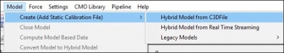
- Select Hybrid Model from C3DFile
- A dialog titled Select the calibration file for the new model will appear. Select static.c3d and click Open.
- Visual3D will switch to Model Building mode automatically. The 3D viewer will display the average value of the marker locations from the standing file. The dialog bar to the left of the screen will contain a list of segments, which by default will contain only a segment representing the Laboratory.

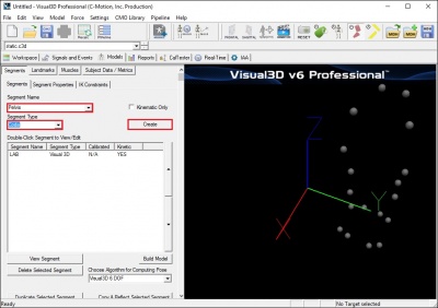
Creating the CODA Pelvis Segment - Step 1a
To construct the CODA Pelvis segment:
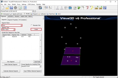
- From the Segment Name box, select Pelvis.
- From the Segment Type box, select Coda.
- Click Create.
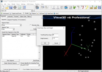
- A dialogue box labeled Enter Body Mass and Height will open because Visual3D needs the subject to be assigned a mass and a height. For this example, Enter 56 kg and 1.77 m, and click OK.
- A dialogue box labeled CODA Segment Markers will open. Select the markers so that they correspond to the figure below. Click Close.
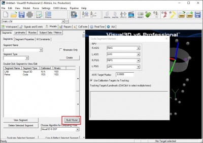
- Click Build Model to build the segment. You should now see a pelvis segment on your standing model. If you do not see the pelvis segment after clicking Build Model, double check the values you entered in the last step.


Bell and Brand Hip Joint Center - Step 2a
The hip joint center calculation is based on a regression equation (Bell and Brand 1989) that will provide estimates of the distance from the pelvic origin to the hip joint center relative to the pelvic coordinate system. Inter-ASIS distance is the only measurement that is needed. The anthropometric section describes inter-ASIS distance measurement. It can be clinically measured or that distance can be calculated from the 3D positions of the ASIS markers. No measurements of leg length or ASIS to GT is needed.
The hip joint center regression equation is defined as:
RIGHT_HIP=(0.36*ASIS_Distance,-0.19*ASIS_Distance,-0.3*ASIS_Distance)
LEFT_HIP=(-0.36*ASIS_Distance,-0.19*ASIS_Distance,-0.3*ASIS_Distance)
Estimates for the Right and Left Hip Joint Center are represented as Landmarks that are created automatically when the Coda_Pelvis segment is created. To view right and left hip joint centers, click on the Landmarks TAB. In the image below, the Landmarks are shown in blue.

- Note: that if the ASIS markers have been placed medial or lateral to the palpated landmark because the subject is obese or because the markers cannot be placed at these locations, it is important to measure the inter-ASIS distance and enter this value into the Subject Data/Metrics TAB. If this is not done, then the hip joint center calculations will be incorrect.
Enter Subject Measurements
The CODA pelvis does not require direct measurement. However, the conventional gait model does require measurement of knee and ankle width. To enter those measurements in Visual 3D, the user must create a Subject Data Metric for that measurement.
- Click on Subject Data/Metrics tab
- Click Add New Item
- Type in RKNEEWIDTH in Name
- Type in 0.099 in Value of Expression
- Click on OK

RKNEEWIDTH should now appear in the list. Using the above steps, continue to enter the following subject data metrics:
- LKNEEWIDTH in Name and 0.1 in Value of Expression
- RANKLEWIDTH in Name and 0.066 in Value of Expression
- LANKLEWIDTH in Name and 0.069 in Value of Expression
- MARKER_Radius in Name and 0.012 in Value of Expression
The Subject Data/Metrics should look like the image below.

Create Thigh Segments - Steps 3b and 4b
To create the right thigh segment:
- Click on Segments tab
- From the Segment Name box, select Right Thigh.
- From the Segment Type box, select Visual 3D.
- Click Create.

A dialog will open that will allow us to define the segment. To create a thigh segment Visual3D treats the thigh as a geometrical primitive (conical frustrum). The proximal and distal ends of the segment must be defined.
- In the Define Proximal Joint and Radius section, select RIGHT_HIP for the Joint.
- In the Proximal Radius box, enter .089. The proximal radius is the geometrical radius of the proximal end of the thigh. You can use calipers to measure this or you can approximate this measure as one quarter of the distance between the greater trochanters.
- In the Define Distal Joint and Radius section, select RFLE for the Lateral.
- In the Distal Radius box, enter 0.5*RKNEEWIDTH+MARKER_RADIUS
- In the Extra Target to Define Orientation section, select Lateral for the Location. and RTH for the marker.
- In the Select Tracking Targets, click on RIGHT_HIP, RFLE, and RTH
- Click on Build Model
You should now see a thigh segment on your standing model. If you do not see the thigh segment after clicking Build Model, double check the values you entered in the last step.

To create the left thigh segment:
- Click on Close tab
- From the Segment Name box, select Left Thigh.
- From the Segment Type box, select Visual 3D.
- Click Create.
- In the Define Proximal Joint and Radius section, select LEFT_HIP for the Joint.
- In the Proximal Radius box, enter .089.
- In the Define Distal Joint and Radius section, select LFLE for the Lateral.
- In the Distal Radius box, enter 0.5*LKNEEWIDTH+MARKER_RADIUS
- In the Extra Target to Define Orientation section, select Lateral for the Location. and LTH for the marker.
- In the Select Tracking Targets, click on LEFT_HIP, LFLE, and LTH
- Click on Build Model
You should now see both thigh segments on your standing model.

Create Knee Joint Centers
The knee joint center of the Conventional Gait Model is assumed to be fixed in both the femur and tibia. It's location is half the knee width and half a marker diameter medial to the center of the lateral epicondyle marker in the plane of the femoral segment.
When we constructed the thigh segments, we used these calculations to define the distal joint and radius. Now we can explicitly define the knee joint center by creating a landmark at the distal end of the thigh segment.
To create the right knee joint center landmark:
- Click on the Landmarks TAB
- Click on Add New Landmark tab
- In the Landmark Name box, enter RIGHT_KNEE
- From the Existing Segment box, select Right Thigh.
- From the Offset Using the Following AP/ML/Axial Offsets box, in the AXIAL enter -1
- Check the Offset by Percent (1.0=100%) (Meters when not checked)
- Click Apply.

To create the left knee joint center landmark:
- Click on the Landmarks TAB
- Click on Add New Landmark tab
- In the Landmark Name box, enter LEFT_KNEE
- From the Existing Segment box, select Left Thigh.
- From the Offset Using the Following AP/ML/Axial Offsets box, in the AXIAL enter -1
- Check the Offset by Percent (1.0=100%) (Meters when not checked)
- Click Apply.
In the image below, the Landmarks are shown in blue.

Create Shank Segments - Steps 5b
To create the right shank segment:
- Click on Segments tab
- From the Segment Name box, select Right Shank.
- From the Segment Type box, select Visual 3D.
- Click Create.
A dialog will open that will allow us to define the segment. To create a shank segment:
- In the Define Proximal Joint and Radius section, select RFLE for the Lateral.
- In the Define Proximal Joint and Radius section, select RIGHT_KNEE for the Joint.
- In the Define Distal Joint and Radius section, select RFAL for the Lateral.
- In the Distal Radius box, enter 0.5*RANKLEWIDTH+MARKER_RADIUS
- In the Select Tracking Targets, click on RIGHT_KNEE, RFAL, RFLE, and RSK
- Click on Build Model
You should now see a shank segment on your standing model. If you do not see the shank segment after clicking Build Model, double check the values you entered in the last step.

To create the left shank segment:
- Click on Close tab
- From the Segment Name box, select Left Shank.
- From the Segment Type box, select Visual 3D.
- Click Create.
- In the Define Proximal Joint and Radius section, select LFLE for the Lateral.
- In the Define Proximal Joint and Radius section, select LEFT_KNEE for the Joint.
- In the Define Distal Joint and Radius section, select LFAL for the Lateral.
- In the Distal Radius box, enter 0.5*LANKLEWIDTH+MARKER_RADIUS
- In the Select Tracking Targets, click on LEFT_KNEE, LFAL, LFLE, and LSK
- Click on Build Model
You should now see both shank segments on your standing model.

Create Ankle Joint Centers
As with the knee, the ankle joint center is assumed to be fixed in both the tibia and foot. It's location is half the ankle width and half a marker diameter medial to the center of the lateral malleolus marker in the plane of the tibial segment.
When we constructed the shank segments, we used these calculations to define the distal joint and radius. Now we can explicitly define the knee joint center by creating a landmark at the distal end of the thigh segment.
To create the right ankle joint center landmark:
- Click on the Landmarks TAB
- Click on Add New Landmark tab
- In the Landmark Name box, enter RIGHT_ANKLE
- From the Existing Segment box, select Right Shank.
- From the Offset Using the Following AP/ML/Axial Offsets box, in the AXIAL enter -1
- Check the Offset by Percent (1.0=100%) (Meters when not checked)
- Click Apply.

To create the left ankle joint center landmark:
- Click on the Landmarks TAB
- Click on Add New Landmark tab
- In the Landmark Name box, enter LEFT_ANKLE
- From the Existing Segment box, select Left Shank.
- From the Offset Using the Following AP/ML/Axial Offsets box, in the AXIAL enter -1
- Check the Offset by Percent (1.0=100%) (Meters when not checked)
- Click Apply.
In the image below, the Landmarks are shown in blue.

Create Foot Segments
To create the right shank segment:
- Click on Segments tab
- From the Segment Name box, select Right Foot.
- From the Segment Type box, select Visual 3D.
- Click Create.
A dialog will open that will allow us to define the segment. To create a shank segment:
- In the Define Proximal Joint and Radius section, select RFAL for the Lateral.
- In the Define Proximal Joint and Radius section, select RIGHT_ANKLE for the Joint.
- In the Define Distal Joint and Radius section, select RSMH for the Joint.
- In the Distal Radius box, enter 0.06
- In the Select Tracking Targets, click on RIGHT_ANKLE, RFAL, and RSMH
- Click on Build Model
You should now see a foot segment on your standing model. If you do not see the foot segment after clicking Build Model, double check the values you entered in the last step.

To create the left foot segment:
- Click on Close tab
- From the Segment Name box, select Left Foot.
- From the Segment Type box, select Visual 3D.
- Click Create.
- In the Define Proximal Joint and Radius section, select LFAL for the Lateral.
- In the Define Proximal Joint and Radius section, select LEFT_ANKLE for the Joint.
- In the Define Distal Joint and Radius section, select LSMH for the Joint.
- In the Distal Radius box, enter 0.06
- In the Select Tracking Targets, click on LEFT_ANKLE, LFAL, and LSMH
- Click on Build Model
You should now see both foot segments on your standing model.

Example 2: with HH pelvis & no KAD - Steps:1b,2c,3b,4b,5b
This section will detail the construction of the following version of the Conventional Gait Model. Click [Conventional Gait Example 2] to download example files.
- HH pelvis, Davis HJC with ASIS to GT regression, no KAD, no medial knee or ankle markers - Steps: 1b,2c,3b,4b,5b
We begin constructing the Conventional Gait Model by using the static standing trial.
- From the Model menu, select Create (Add Static Calibration File)
- Select Hybrid Model from C3DFile
- A dialog titled Select the calibration file for the new model will appear. Select Normal Static no KAD Trial.c3d and click Open.
- Visual3D will switch to Model Building mode automatically. The 3D viewer will display the average value of the marker locations from the standing file. The dialog bar to the left of the screen will contain a list of segments, which by default will contain only a segment representing the Laboratory.
Creating the HH Pelvis Segment - Step 1b
To construct the HH Pelvis (Davis) segment:
- From the Segment Name box, select Pelvis.
- From the Segment Type box, select Helen Hayes.
- Click Create.
- A dialogue box labeled Enter Body Mass and Height will open because Visual3D needs the subject to be assigned a mass and a height. For this example, Enter 56 kg and 1.77 m, and click OK.
- A dialogue box labeled Helen Hayes/Derived Segment Markers will open. Select the markers so that they correspond to the figure below. Click Close.
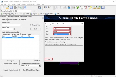
- Click Build Model to build the segment. You should now see a pelvis segment on your standing model. If you do not see the pelvis segment after clicking Build Model, double check the values you entered in the last step.


Enter Subject Measurements
When Visual 3D creates the HH Pelvis, Subject Data/Metrics are created for the model. Since the hip joint center calculation for HH Pelvis model is based on inter-ASIS distance, leg length, and ASIS to GT distance, these values need to be entered into the Subject Data/Metrics Tab. In addition, knee and ankle width Subject Data/Metrics need to be created and entered.
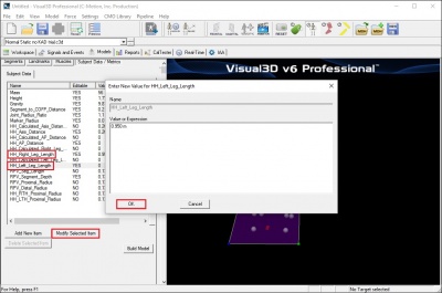
Enter the values by selecting Modify Selected Item for each of the items below:
- Enter .950 m for HH_Right_Leg_Length
- Enter .950 m for HH_Left_Leg_Length
- In this example, the values for inter-ASIS distance will be calculated from the 3D markers positions of the ASIS's and the ASIS to GT distance will be calculated from a regression equation. There is no need to enter or change values for these variables. If a clinically measured distance is not entered, Visual 3D defaults to the calculated variables.
- Click Build Model to build the segment. The hip joint centers should now be calculated properly. For further disussion on the hip joint center calculations see the Joint Center Calculations section.

To add Knee and Ankle width:
- Click Add New Item
- Type in Right_Knee_Width in Name
- Type in 0.110 in Value of Expression
- Click on OK
Using the above steps, continue to enter the following subject data metrics:
- Left_Knee_Width in Name and 0.110 in Value of Expression
- Right_Ankle_Width in Name and 0.080 in Value of Expression
- Left_Ankle_Width in Name and 0.080 in Value of Expression
The Subject Data/Metrics should look like the image below.

HJC Regression Without Clinical Measurement of ASIS to GT (Davis 1991)
The hip joint center calculation is based on a regression equation (Davis 1991) that will provide estimates of the distance from the pelvic origin to the hip joint center relative to the pelvic coordinate system. Measurements of leg length, anteroposterior ASIS to Greater Trochanter distance, and inter-ASIS distance are needed. The anthropometric section describes the measurements for leg length and inter-ASIS distance.
If no clinical measurement of anteroposterior distance between the ASIS to Greater Trochanter is taken, then the equation below will be used:
Bilateral anteroposterior distance= 0.1288*Leg Length-0.04856
The regression equation is follows:
Hip X = -S (C sin(theta)-0.5*distASIS)
Hip Y = (-Xdis-Rmarker) cos(beta)+ C cos(theta) sin(beta)
Hip Z = (-Xdis-Rmarker) sin(beta)- C cos(theta) cos(beta)

Where:
C = 0.115*LegLength - 0.0153 (in meters)

theta = 28.4*PI/180.0

beta = 18.0*PI/180.0

distASIS = ASIS to ASIS distance, measured during clinical exam

Xdis = anterior/posterior component of the ASIS/hip center distance in the sagittal plane of the
       pelvis and measured during the clinical exam

If Xdis not measured:
 Xdis = 0.1288*LegLength - 0.04856

Rmarker = marker Radius (in meters)

S = +1 for the right side and -1 for the left side
Estimates for the Right and Left Hip Joint Center are represented as Landmarks that are created automatically when the Helen Hayes (Davis) Pelvis segment is created. To view right and left hip joint centers, click on the Landmarks TAB. In the image below, the Landmarks are shown in blue.
File:Helen Hayes Pelvis Joint Centers Calc ASIS to GT1.jpg
- Note: that if the ASIS markers have been placed medial or lateral to the palpated landmark because the subject is obese or because the markers cannot be placed at these locations, it is important to measure the inter-ASIS distance and enter this value into the Subject Data/Metrics TAB. If this is not done, then the hip joint center calculations will be incorrect.
Create Thigh Segments - Steps 3b and 4b
To create the right thigh segment:
- Click on Segments tab
- From the Segment Name box, select Right Thigh.
- From the Segment Type box, select Visual 3D.
- Click Create.
A dialog will open that will allow us to define the segment. To create a thigh segment Visual3D treats the thigh as a geometrical primitive (conical frustrum). The proximal and distal ends of the segment must be defined.
- In the Define Proximal Joint and Radius section, select HH_RIGHT_HIP for the Joint.
- In the Proximal Radius box, enter .089. The proximal radius is the geometrical radius of the proximal end of the thigh. You can use calipers to measure this or you can approximate this measure as one quarter of the distance between the greater trochanters.
- In the Define Distal Joint and Radius section, select RFLE for the Lateral.
- In the Distal Radius box, enter 0.5*Right_Knee_Width+Marker_Radius
- In the Extra Target to Define Orientation section, select Lateral for the Location. and RTH for the marker.
- In the Select Tracking Targets, click on HH_RIGHT_HIP, RFLE, and RTH
- Click on Build Model
You should now see a thigh segment on your standing model. If you do not see the thigh segment after clicking Build Model, double check the values you entered in the last step.
To create the left thigh segment:
- Click on Close tab
- From the Segment Name box, select Left Thigh.
- From the Segment Type box, select Visual 3D.
- Click Create.
- In the Define Proximal Joint and Radius section, select HH_LEFT_HIP for the Joint.
- In the Proximal Radius box, enter .089.
- In the Define Distal Joint and Radius section, select LFLE for the Lateral.
- In the Distal Radius box, enter 0.5*Left_Knee_Width+Marker_Radius
- In the Extra Target to Define Orientation section, select Lateral for the Location. and LTH for the marker.
- In the Select Tracking Targets, click on HH_LEFT_HIP, LFLE, and LTH
- Click on Build Model
You should now see both thigh segments on your standing model.
Create Knee Joint Centers
The knee joint center of the Conventional Gait Model is assumed to be fixed in both the femur and tibia. It's location is half the knee width and half a marker diameter medial to the center of the lateral epicondyle marker in the plane of the femoral segment.
When we constructed the thigh segments, we used these calculations to define the distal joint and radius. Now we can explicitly define the knee joint center by creating a landmark at the distal end of the thigh segment.
To create the right knee joint center landmark:
- Click on the Landmarks TAB
- Click on Add New Landmark tab
- In the Landmark Name box, enter HH_RIGHT_KNEE
- From the Existing Segment box, select Right Thigh.
- From the Offset Using the Following AP/ML/Axial Offsets box, in the AXIAL enter -1
- Check the Offset by Percent (1.0=100%) (Meters when not checked)
- Click Apply.
To create the left knee joint center landmark:
- Click on the Landmarks TAB
- Click on Add New Landmark tab
- In the Landmark Name box, enter HH_LEFT_KNEE
- From the Existing Segment box, select Left Thigh.
- From the Offset Using the Following AP/ML/Axial Offsets box, in the AXIAL enter -1
- Check the Offset by Percent (1.0=100%) (Meters when not checked)
- Click Apply.
In the image below, the Landmarks are shown in blue.
File:Helen Hayes Knee Joint Center.jpg
Create Shank Segments - Steps 5b
To create the right shank segment:
- Click on Segments tab
- From the Segment Name box, select Right Shank.
- From the Segment Type box, select Visual 3D.
- Click Create.
A dialog will open that will allow us to define the segment. To create a shank segment:
- In the Define Proximal Joint and Radius section, select HH_RIGHT_KNEE for the Joint.
- In the Proximal Radius box, enter 0.5*Right_Knee_Width+Marker_Radius
- In the Define Distal Joint and Radius section, select RFAL for the Lateral.
- In the Distal Radius box, enter 0.5*Right_Ankle_Width+Marker_Radius
- In the Extra Target to Define Orientation section, select Lateral for the Location. and RSK for the marker.
- In the Select Tracking Targets, click on HH_RIGHT_KNEE, RFAL, RFLE, and RSK
- Click on Build Model
You should now see a shank segment on your standing model. If you do not see the shank segment after clicking Build Model, double check the values you entered in the last step.
File:HH Right Shank segment1.jpg
To create the left shank segment:
- Click on Close tab
- From the Segment Name box, select Left Shank.
- From the Segment Type box, select Visual 3D.
- Click Create.
- In the Define Proximal Joint and Radius section, select HH_LEFT_KNEE for the Joint.
- In the Proximal Radius box, enter 0.5*Left_Knee_Width+Marker_Radius
- In the Define Distal Joint and Radius section, select LFAL for the Lateral.
- In the Distal Radius box, enter 0.5*Left_Ankle_Width+Marker_Radius
- In the Extra Target to Define Orientation section, select Lateral for the Location. and LSK for the marker.
- In the Select Tracking Targets, click on HH_LEFT_KNEE, LFAL, LFLE, and LSK
- Click on Build Model
You should now see both shank segments on your standing model.
Create Ankle Joint Centers
As with the knee, the ankle joint center is assumed to be fixed in both the tibia and foot. It's location is half the ankle width and half a marker diameter medial to the center of the lateral malleolus marker in the plane of the tibial segment.
When we constructed the shank segments, we used these calculations to define the distal joint and radius. Now we can explicitly define the knee joint center by creating a landmark at the distal end of the thigh segment.
To create the right ankle joint center landmark:
- Click on the Landmarks TAB
- Click on Add New Landmark tab
- In the Landmark Name box, enter HH_RIGHT_ANKLE
- From the Existing Segment box, select Right Shank.
- From the Offset Using the Following AP/ML/Axial Offsets box, in the AXIAL enter -1
- Check the Offset by Percent (1.0=100%) (Meters when not checked)
- Click Apply.
To create the left knee joint center landmark:
- Click on the Landmarks TAB
- Click on Add New Landmark tab
- In the Landmark Name box, enter HH_LEFT_ANKLE
- From the Existing Segment box, select Left Shank.
- From the Offset Using the Following AP/ML/Axial Offsets box, in the AXIAL enter -1
- Check the Offset by Percent (1.0=100%) (Meters when not checked)
- Click Apply.
In the image below, the Landmarks are shown in blue.
File:Helen Hayes Ankle Joint Center.jpg
Create Foot Segments
To create the right shank segment:
- Click on Segments tab
- From the Segment Name box, select Right Foot.
- From the Segment Type box, select Visual 3D.
- Click Create.
A dialog will open that will allow us to define the segment. To create a shank segment:
- In the Define Proximal Joint and Radius section, select RFAL for the Lateral.
- In the Define Proximal Joint and Radius section, select HH_RIGHT_ANKLE for the Joint.
- In the Define Distal Joint and Radius section, select RSMH for the Joint.
- In the Distal Radius box, enter 0.06
- In the Select Tracking Targets, click on HH_RIGHT_ANKLE, RFAL, RSMH, and RVMH
- Click on Build Model
You should now see a foot segment on your standing model. If you do not see the foot segment after clicking Build Model, double check the values you entered in the last step.
File:CODA Right Foot segment.jpg
To create the left foot segment:
- Click on Close tab
- From the Segment Name box, select Left Foot.
- From the Segment Type box, select Visual 3D.
- Click Create.
- In the Define Proximal Joint and Radius section, select LFAL for the Lateral.
- In the Define Proximal Joint and Radius section, select HH_LEFT_ANKLE for the Joint.
- In the Define Distal Joint and Radius section, select LSMH for the Joint.
- In the Distal Radius box, enter 0.06
- In the Select Tracking Targets, click on HH_LEFT_ANKLE, LFAL, LSMH, and LVMH
- Click on Build Model
You should now see both foot segments on your standing model.
Example 3: with HH Pelvis with KAD - Steps:1b,2b,3a,4b,5a
This section will detail the construction of the following version of the Conventional Gait Model. Click [Conventional Gait Example 3] to download example files.
- HH pelvis, Davis HJC with clinically measured ASIS to GT distance, with KAD, no medial knee, ankle markers - Steps:1b,2b,3a,4b,5a
We begin by using the static standing trial.
- From the Model menu, select Create (Add Static Calibration File)
- Select Hybrid Model from C3DFile
- A dialog titled Select the calibration file for the new model will appear. Select Normal Static with KAD trial.c3d and click Open.
- Visual3D will switch to Model Building mode automatically. The 3D viewer will display the average value of the marker locations from the standing file. The dialog bar to the left of the screen will contain a list of segments, which by default will contain only a segment representing the Laboratory.
Creating the HH Pelvis Segment
To construct the HH Pelvis (Davis) segment:
- From the Segment Name box, select Pelvis.
- From the Segment Type box, select Helen Hayes.
- Click Create.
File:HH Pelvis KAD.jpg - A dialogue box labeled Enter Body Mass and Height will open because Visual3D needs the subject to be assigned a mass and a height. For this example, Enter 56 kg and 1.77 m, and click OK.
- A dialogue box labeled Helen Hayes/Derived Segment Markers will open. Select the markers so that they correspond to the figure below. Click Close.
File:HH Pelvis KAD Markers.jpg - Click Build Model to build the segment. You should now see a pelvis segment on your standing model. If you do not see the pelvis segment after clicking Build Model, double check the values you entered in the last step.
Enter Subject Measurements
When Visual 3D creates the HH Pelvis, Subject Data/Metrics are created for the model. Since the hip joint center calculation for HH Pelvis model is based on inter-ASIS distance, leg length, and ASIS to GT distance, these values need to be entered into the Subject Data/Metrics Tab.
Enter the values by selecting Modify Selected Item for each of the items below:
- Enter 0.950 m for HH_Right_Leg_Length
- Enter 0.950 m for HH_Left_Leg_Length
- In this example, the values for inter-ASIS distance will be calculated from the 3D markers positions of the ASIS's
- The ASIS to GT distance is measured clinically. Enter 0.074 for HH_AP_Distance
File:HH Subject Data Metrics KAD.jpg - Click Build Model to build the segment. The hip joint centers should now be calculated properly. For further disussion on the hip joint center calculations see the Joint Center Calculations section.
HJC Regression with Clinical Measurement of ASIS to GT (Davis 1991)
The hip joint center calculation is based on a regression equation (Davis 1991) that will provide estimates of the distance from the pelvic origin to the hip joint center relative to the pelvic coordinate system. Measurements of leg length, anteroposterior ASIS to Greater Trochanter distance, and inter-ASIS distance are needed. The anthropometric section describes the measurements for leg length, anteroposterior ASIS to Greater Trochanter distance, and inter-ASIS distance. The regression equation was shown in the Hip joint center calculations in Example 2.
Estimates for the Right and Left Hip Joint Center are represented as Landmarks that are created automatically when the Helen Hayes (Davis) Pelvis segment is created. To view right and left hip joint centers, click on the Landmarks TAB. In the image below, the Landmarks are shown in blue.
File:Helen Hayes Pelvis Joint Centers Meas ASIS to GT.jpg
- Note: that if the ASIS markers have been placed medial or lateral to the palpated landmark because the subject is obese or because the markers cannot be placed at these locations, it is important to measure the inter-ASIS distance and enter this value into the Subject Data/Metrics TAB. If this is not done, then the hip joint center calculations will be incorrect.
Create KAD Segments - Steps 3a
We must make a virtual segment (kinematic only) for the KAD. To create a Kinematic Only right KAD segment:
- Click on Segments tab
- From the Segment Name box, select Right KAD.
- From the Segment Type box, select Visual 3D.
- Check the Kinematic Only box
- Click Create.
File:HH KAD segment1.jpg - A dialogue box labeled Helen Hayes/Derived Segment Markers will open. Select the markers so that they correspond to the figure below. Click Close.
File:HH KAD segment markers1.jpg - Click Build Model to build the segment. You should now see the KAD segment coordinate system on your standing model. If you do not see the KAD coordinate system after clicking Build Model, double check the values you entered in the last step.
File:HH KAD segments.jpg
To create the left KAD segment:
- Click on Segments tab
- From the Segment Name box, select Left KAD.
- From the Segment Type box, select Visual 3D.
- Click Create.
- A dialogue box labeled Helen Hayes/Derived Segment Markers will open. Select the markers similar to step 6 above. Click Close.
- Click Build Model to build the segment. You should now see the KAD segment coordinate system on your standing model. If you do not see the KAD coordinate system after clicking Build Model, double check the values you entered in the last step.
File:HH KAD segment Full1.jpg
Note: Many laboratories have taken to replacing the 25 mm markers with smaller markers, in an erroneous assumption that it would be a good idea to have all markers used on the body and the KAD to be the same size. This actually introduces an error in the assumptions of how the KAD is used. If this is done, the user must be careful to accommodate this change to the original assumptions.
Edit Subject Metrics and Landmarks
When the KAD segments are created, Visual 3D creates the Knee and Ankle width subject metrics from default values. These need to be edited to reflect the current subject. #Click on Subject Data/Metrics tab and enter the values by selecting Modify Selected Item for each of the items below:
- Enter 0.110 m for Right_Knee_Width
- Enter 0.110 m for Left_Knee_Width
- Enter 0.080 m for Right_Ankle_Width
- Enter 0.080 m for Left_Ankle_Width
In addition, when the KAD segments are created, Visual 3D also creates virtual points or Landmarks for the knee. These need to be edited to reflect our tutorial marker set labels.
- Enter 'RFLE for HH_RIGHT_KNEE_FROM_KAD
- Enter 'LFLE for HH_LEFT_KNEE_FROM_KAD
The Subject Data/Metrics should look like the image below.
File:HH Subject Data Metrics KAD All1.jpg
Create Thigh Segments - Steps 4b
To create the right thigh segment:
- Click on Segments tab
- From the Segment Name box, select Right Thigh.
- From the Segment Type box, select Visual 3D.
- Click Create.
A dialog will open that will allow us to define the segment. To create a thigh segment Visual3D treats the thigh as a geometrical primitive (conical frustrum). The proximal and distal ends of the segment must be defined.
- In the Define Proximal Joint and Radius section, select HH_RIGHT_HIP for the Joint.
- In the Proximal Radius box, enter .089. The proximal radius is the geometrical radius of the proximal end of the thigh. You can use calipers to measure this or you can approximate this measure as one quarter of the distance between the greater trochanters.
- In the Define Distal Joint and Radius section, select HH_RIGHT_KNEE_FROM_KAD for the Joint.
- In the Distal Radius box, enter 0.5*Right_Knee_Width+Marker_Radius
- In the Extra Target to Define Orientation section, select Lateral for the Location. and RFLE for the marker.
- In the Select Tracking Targets, click on HH_RIGHT_HIP, HH_RIGHT_KNEE_FROM_KAD, RFLE, and RTH
- Click on Build Model
You should now see a thigh segment on your standing model. If you do not see the thigh segment after clicking Build Model, double check the values you entered in the last step. File:HH KAD Thigh segment1.jpg
To create the left thigh segment:
- Click on Segments tab
- From the Segment Name box, select Left Thigh.
- From the Segment Type box, select Visual 3D.
- Click Create.
In the dialog enter:
- In the Define Proximal Joint and Radius section, select HH_LEFT_HIP for the Joint.
- In the Proximal Radius box, enter .089. The proximal radius is the geometrical radius of the proximal end of the thigh. You can use calipers to measure this or you can approximate this measure as one quarter of the distance between the greater trochanters.
- In the Define Distal Joint and Radius section, select HH_LEFT_KNEE_FROM_KAD for the Joint.
- In the Distal Radius box, enter 0.5*Left_Knee_Width+Marker_Radius
- In the Extra Target to Define Orientation section, select Lateral for the Location. and LFLE for the marker.
- In the Select Tracking Targets, click on HH_LEFT_KNEE_FROM_KAD, HH_LEFT_HIP, LFLE, and LTH
- Click on Build Model
File:HH KAD Thigh segment all.jpg
Knee Joint Centers
The knee joint center of the Conventional Gait Model is assumed to be fixed in both the femur and tibia. It's location is half the knee width and half a marker diameter medial to the center of the lateral epicondyle marker in the plane of the femoral segment. When we constructed the KAD thigh segments, we used these calculations to define the distal joint and radius. The knee joint center was explicitly defined the by creating a landmark at the distal end of the thigh segment. Those markers are HH_LEFT_KNEE_FROM_KAD and HH_RIGHT_KNEE_FROM_KAD. To view the knee joint center landmarks, click on the Landmarks TAB.
Create Shank Segments - Steps 5b
To create the right shank segment:
- Click on Segments tab
- From the Segment Name box, select Right Shank.
- From the Segment Type box, select Visual 3D.
- Click Create.
A dialog will open that will allow us to define the segment. To create a shank segment:
- In the Define Proximal Joint and Radius section, select HH_RIGHT_KNEE_FROM_KAD for the Joint.
- In the Proximal Radius box, enter 0.5*Right_Knee_Width+Marker_Radius
- In the Define Distal Joint and Radius section, select RFAL for the Lateral.
- In the Distal Radius box, enter 0.5*Right_Ankle_Width+Marker_Radius
- In the Extra Target to Define Orientation section, select Lateral for the Location. and RSK for the marker.
- In the Select Tracking Targets, click on HH_RIGHT_KNEE_FROM_KAD, RFAL, RFLE, and RSK
- Click on Build Model
You should now see a shank segment on your standing model. If you do not see the shank segment after clicking Build Model, double check the values you entered in the last step.
File:HH Right Shank segment1.jpg
To create the left shank segment:
- Click on Close tab
- From the Segment Name box, select Left Shank.
- From the Segment Type box, select Visual 3D.
- Click Create.
- In the Define Proximal Joint and Radius section, select HH_LEFT_KNEE_FROM_KAD for the Joint.
- In the Proximal Radius box, enter 0.5*Left_Knee_Width+Marker_Radius
- In the Define Distal Joint and Radius section, select LFAL for the Lateral.
- In the Distal Radius box, enter 0.5*Left_Ankle_Width+Marker_Radius
- In the Extra Target to Define Orientation section, select Lateral for the Location. and LSK for the marker.
- In the Select Tracking Targets, click on HH_LEFT_KNEE_FROM_KAD, LFAL, LFLE, and LSK
- Click on Build Model
You should now see both shank segments on your standing model.
Create Ankle Joint Centers
As with the knee, the ankle joint center is assumed to be fixed in both the tibia and foot. It's location is half the ankle width and half a marker diameter medial to the center of the lateral malleolus marker in the plane of the tibial segment.
When we constructed the shank segments, we used these calculations to define the distal joint and radius. Now we can explicitly define the knee joint center by creating a landmark at the distal end of the thigh segment.
To create the right ankle joint center landmark:
- Click on the Landmarks TAB
- Click on Add New Landmark tab
- In the Landmark Name box, enter HH_RIGHT_ANKLE
- From the Existing Segment box, select Right Shank.
- From the Offset Using the Following AP/ML/Axial Offsets box, in the AXIAL enter -1
- Check the Offset by Percent (1.0=100%) (Meters when not checked)
- Click Apply.
To create the left knee joint center landmark:
- Click on the Landmarks TAB
- Click on Add New Landmark tab
- In the Landmark Name box, enter HH_LEFT_ANKLE
- From the Existing Segment box, select Left Shank.
- From the Offset Using the Following AP/ML/Axial Offsets box, in the AXIAL enter -1
- Check the Offset by Percent (1.0=100%) (Meters when not checked)
- Click Apply.
In the image below, the Landmarks are shown in blue.
File:Helen Hayes Ankle Joint Center.jpg
Create Foot Segments
To create the right shank segment:
- Click on Segments tab
- From the Segment Name box, select Right Foot.
- From the Segment Type box, select Visual 3D.
- Click Create.
A dialog will open that will allow us to define the segment. To create a shank segment:
- In the Define Proximal Joint and Radius section, select RFAL for the Lateral.
- In the Define Proximal Joint and Radius section, select HH_RIGHT_ANKLE for the Joint.
- In the Define Distal Joint and Radius section, select RSMH for the Joint.
- In the Distal Radius box, enter 0.06
- In the Select Tracking Targets, click on HH_RIGHT_ANKLE, RFAL, and RSMH
- Click on Build Model
You should now see a foot segment on your standing model. If you do not see the foot segment after clicking Build Model, double check the values you entered in the last step.
File:CODA Right Foot segment.jpg
To create the left foot segment:
- Click on Close tab
- From the Segment Name box, select Left Foot.
- From the Segment Type box, select Visual 3D.
- Click Create.
- In the Define Proximal Joint and Radius section, select LFAL for the Lateral.
- In the Define Proximal Joint and Radius section, select HH_LEFT_ANKLE for the Joint.
- In the Define Distal Joint and Radius section, select LSMH for the Joint.
- In the Distal Radius box, enter 0.06
- In the Select Tracking Targets, click on HH_LEFT_ANKLE, LFAL, and LSMH
- Click on Build Model
You should now see both foot segments on your standing model.
Summary
This tutorial walked you through some of the variations of the conventional gait model, discussed marker placement issues, and gave you 3 examples that you constructed in Visual 3D. The tutorial was not meant to be comprehensive and some variations of the model are not addressed namely these listed below:
- Constructing virtual foot segment in Visual 3D for which the alignment during the standing trial yields the desired joint angle.
- Rotation of thigh segments by entering in a rotation value
- Rotating tibial segments by entering in a tibial torsion rotation offset, meaning that the clinician measures the transmalleor axis on the table and enters in the value.
- Using medial knee markers to define the knee flexion/ext axis
- Using medial ankle markers to define the transmalleolar axis
References
Bell AL, Pederson DR, and Brand RA (1989) Prediction of hip joint center location from external landmarks. Human Movement Science. 8:3-16
Bell AL, Pedersen DR, Brand RA (1990) A Comparison of the Accuracy of Several hip Center Location Prediction Methods. J Biomech. 23, 617-621.
Davis RB, Ounpuu S, Tyburski D, Gage JR. (1991) "A Gait Analysis Data Collection and Reduction Technique." Human Movement Science 10: 575-587.
Kadaba MP, Ramakrishnan HK, Wootten ME (1990) "Measurement of Lower Extremity Kinematics During Level Walking." J. Orthopedic Research8: 383-392.
Serge van Sint Jan "Color Atlas of Skeletal Landmark Definitions: Guidelines for Reproducible Manual and Virtual Palpations" 2007 - Churchill Livingstone
- ↑ 1.0 1.1 1.2 Leardini, A., M.G. Benedetti, L. Berti, D. Bettinelli, R. Nativo, and S. Giannini. "Rear-foot, Mid-foot and Fore-foot Motion during the Stance Phase of Gait." Gait & Posture 25 (2007): 453-55
- ↑ 2.0 2.1 2.2 Serge van Sint Jan "Color Atlas of Skeletal Landmark Definitions: Guidelines for Reproducible Manual and Virtual Palpations" 2007 - Churchill Livingstone