The Math of Principal Component Analysis (PCA)

note: this page is under construction

The mathematical principles of PCA shown are from the Research Methods in Biomechanics Textbook, chapter 14 [1].

New technology allows researchers to generate large quantities of data, whether it be time-series data, or any other waveform data that we commonly see in biomechanics research. And what is common amongst all these forms of data is that they are highly dimensional [1]. With new technologies like [Markerless], we are collecting so much more data that trying to make meaningful comparisons is difficult to understand and to do computationally.

In the research methods in biomechanics text, it is emphasized that the basic point of looking at methods of processing waveform data is that no matter the type of research questions that a biomechanist is trying to answer, transforming our data into smaller forms makes it more manageable and useful for analysis. Prior to being able to make meaningful comparisons, we want to reduce the amount of data and not lose any important discriminatory information that may be crucial to our comparisons [1].

Traditional approaches of extracting features from waveform data (max, min, range, etc.) result in a lose of so much temporal information in the waveform, leading to a large reduction in data and discarded information. Additionally, varying definitions of these discrete parameters across the field lead to inconsistent conclusions, and these measures may not always be definitive in certain populations [1]. One such example mentioned in the text found that knee adduction angles in patients with OA don’t have definitive peaks, and thus finding max and min angles is meaningless [2].

PCA

PCA is an orthogonal decomposition technique that computes and extracts a unique set of basis functions from the waveforms based on the variation that is present in the waveform data [1].

Waveform Data

Waveform data can be represented in matrix form , where the rows are the time series waveforms for each subject, and the columns are particular points within the waveform (n = subjects, p = points) [1].

Covariance Matrix

To define variation in the waveform matrix, X, based on how the data changes over time, and between subjects (n) at each point in time (p), we look at the covariance matrix, S. The diagonal elements of the covariance matrix are the variation at each instance in the data. The off-diagonal elements represent the variation in each pair of instances. If the covariance values are non-zero, this means there is a linear relationship between the variables. If the off-diagonal values of S are non-zero, this means that the columns of the original data X are correlated. However, principal components are orthogonal, independent features of the original data, and thus we look for principal components that have a covariance matrix with off-diagonal components equal to zero [1].

To transform the original data set covariance matrix, S, into a principal component covariance matrix, D, diagonalization is used, where U is an orthogonal transformation matrix. U transforms the data into the new coordinate system, which are the coordinates of the principal components [1].

U'SU = D

Loading Vectors

The columns of matrix U are the eigenvectors of the covariance matrix S. Many people refer to these eigenvectors as the principal component's loading vectors [1].

The matrix D is a diagonal covariance matrix. The individual elements of D are the individual measures of variance for each principal component, and are the eigenvalues of the covariance matrix S [1].

See also the PCA loading vector graph.

Principal Components

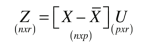
Finally, we use the matrix U to transform out original data matrix into orthogonal principal components (uncorrelated) [1].

The columns of Z are the principal components (linear combinations of the underlying waveform data), while the individual components are the PC scores [1].

See also: Scatter-plotting workspace scores and distribution of scores by group for each PC.

Variance Explained

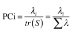
The diagonal elements of D, the eigenvalues, give the variance of each PC. We can represent the total data variation by finding the sum of variances of each variable. The variance are represented by the diagonal components of S, and the sum of the diagonal matrix is called the trace (tr) [1].

tr(S)=tr(D)

From this, we quantify the portion of total variance explained for each PC [1]:

See also: variance explained by each PC individually and variance explained by each PC at each point in the signal's cycle.

Resources

[1] Robertson G., Caldwell G., Hamill J., Kamen G., Whittlesey S., Research Methods in Biomechanics Textbook, 2nd edition ([1])

[2] Deluzio KJ and Astephen JL (2007) Biomechanical features of gait waveform data associated with knee osteoarthritis. An application of principal component anslysis. Gait & Posture 23. 86-93 (pdf)