Sift Tutorial: Outlier Detection with PCA
| Language: | English • français • italiano • português • español |
|---|
This tutorial will show you how to use the outlier detection methods built into Sift, when each method might be appropriate and how to interpret the results. Outlier detection is a key artifact of data analysis, identifying errant data or anomalies that might make further data analysis less effective. Within Sift, there are multiple methods for detecting outliers, but we will be focusing on doing so with PCA data in this tutorial.
Data
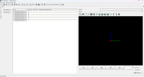
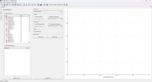
For this tutorial, we will be examining some data from a Visual3D Workshop at a recent ASB meeting. We first need to load the .CMZs into Sift (load from the V3D Workshop folder), and then create and calculate some queries. We will simply use the results from Sifts built in Auto Populate Queries dialog. Your load and explore pages should look as follows:


If you are having trouble with the above instructions, the Sift Tutorials wiki page has many tutorials that will help you out.
Local Outlier Factor
Local Outlier Factor(LOF) is a outlier detection method that uses the local density around data points to determine if a point is an outlier. In this sense it can find outliers that global detection methods would not, as it identifies outliers in local areas.
In Sift, LOF is built upon the PCA module, to find outliers in the PC workspace scores. As such, we will need to create a PCA analysis. To show the benefits of Local Outlier Factor, we will be using the group "HipAngle_Z", as it has a good shape to demonstrate the effectiveness of LOF (multiple clusters of varying density). Specifically, create a PCA on HipAngle_Z with all workspaces selected, 4 PCs calculated, "Use Workspace Mean" unchecked, and named "PCA_HipZ".
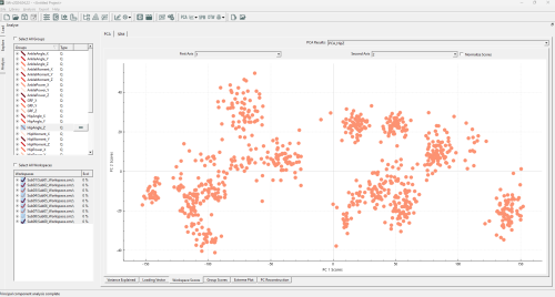
After calculating the PCA Results, the Workspace Scores on the analyse page should look as follows (note that the points are coloured by group. If they were coloured by workspace, you would see many of these clusters correspond to workspaces):

We can see several distinct clusters, in varying positions (and none of which are located at the origin of the plot!). This could cause issues if we were to use "global" outlier detection methods: individual data points may appear to be inliers globally but are actually locally an outlier (i.e. if it is between but not in any of several clusters), or vice-versa, a point (or cluster of points) may be at the edge of the global distribution, but well within a local cluster distribution.
Whichever the situation may be, we are interested in finding outliers in our data, and making a decision upon finding them. We will start by running a LOF calculation. To do so, open the ![]() Outlier Detection Using PCA dropdown on the toolbar, and select "Local Outlier Factor".
Outlier Detection Using PCA dropdown on the toolbar, and select "Local Outlier Factor".
A pop-up window will appear, allowing you to customize some features of the LOF calculation. For this first test, we should set the parameters as below (in the image):
For now, we are looking for outliers from within the entire PCA analysis. We could partition it such that points only calculate their LOF against points in their own group or workspace (which we will show later), but for now we want to look at the whole graph as one, and as such we have selected "Combined Groups".
The number of neighbors is a tuneable parameter within the LOF calculation, and determines how large of a local grouping we will look at. According to the original paper introducing LOF [LINK], a k-value below ~10 can cause issues, so we will at least choose this. They also recommend choosing a k of at least the minimum number of points in a cluster. Looking through our data, a k value > 20 seems reasonable, so we will begin with k=20.
We choose to use 2 PCs, as the workspace scores are presented in 2 dimensions.
Lastly, we choose a manual threshold of 2.0. There is no specific rule for choosing a threshold for inliers vs. outliers, but it should be a number > 1, as below 1 is classified as an inlier. Through iteration, 2.0 is a reasonable value for this data set, as we will see. Generally, we have found that thresholds should be at least > 1.5 to be useful, and to not exclude inliers.
Your LOF dialog should look like this:
Upon running the LOF analysis, you should see several datapoints highlighted:
The highlighted points generally follow what we were hoping to see, any points outside of local clusters are identified as outliers. We see that inliers are determined as such regardless of their cluster density (ex the cluster in the top left is much less dense than others, but is still a valid cluster). We can observe that many of these traces (in the explore page) do not necessarily follow the same trends as the rest of the data, and conclude that they are outliers.
Because Sift has automatically selected the values identified to be outliers, we can easily exclude them on the explore page (if we didn't already do so through the LOF dialog). Simply right click on the explore page graph, and select exclude->exclude data (raw traces).