Sift - OpenBiomechanics Project: Analysis of Baseball Hitters at Different Levels of Competition
| Language: | English • français • italiano • português • español |
|---|
Abstract
The OpenBiomechanics project is an initiative started by Driveline Baseball Research & Development, and provides the general public a marker-based motion capture data set of 100 pitchers and 98 hitters at different levels of competition [1].
The authors provide raw data without any reports or analysis, allowing the general public to use it as they see fit. While numerous articles provide in depth looks into the biomechanics of the baseball swing [2-4], there is a noticeable scarcity in articles that delve into biomechanical disparities between various levels of competition, such as contrasting differences between college and high school baseball players.
This tutorial is designed to demonstrate the use of Sift to analyze the variance in pelvic angular velocity in internal/external rotation between high Blast bat speeds [5] among college and high school baseball players.
Downloads and Relevant Links
Start by downloading the following two zip files.
Please note, these downloads contain a large amount of data. Building CMZs is a slow process, so if you want to speed it up to follow along with building CMZ portion of this tutorial cut the number of datasets under openbiomechanics-main down to 3-5 subjects.
If you want to skip the Build CMZ step of this tutorial and focus on the metadata applications, you can:
- download this pre-built CMZ workspace.
- download the C-Motion Specific Files.
For more technical information about loading metadata, see: Metadata Documentation
Data
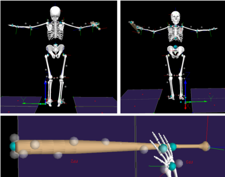
The OpenBiomechanics data set provides cleaned c3d files with 3D kinematic data for 47 body markers, 22 lower limb and pelvic markers, and 25 head, upper limb, and trunk markers; there are also 10 markers placed along the bat. Important metadata that is being considered are highest_playing_level, the level of competition that the subject is currently competing at, and blast_bat_speed_mph_x, the bat speed at contact as measured by Blast Motion sensor in miles per hour. For this tutorial, only the baseball_hitter data set will be analyzed.
Some important contents of the workspace are briefly described below:
- additional_resources: Folder includes additional resources which may be of interest for further exploration, folders you will find include:
- books_articles: Explore scholarly articles pertaining to the field of sports biomechanics, all available as pdfs.
- tutorials: Two tutorials for basic exploration of c3d files using ezc3d package in Python, as well as utilizing ISBS workshop.
- baseball_hitting & baseball_pitching: contains Data, Code, and Imgs folder along with a README.md file. For this tutorial the Data folder is important, but it is worth looking through the other folders.
- Data: c3d is the only folder of interest for this tutorial, it contains all of the folders for each subject with all of their corresponding .c3d files.
Notes:
- If you have downloaded the prebuilt CMZ workspace you will only find baseball_hitting.
Tables below show the Tags, Signals, and Refinements that will be used in this tutorial. These will be seen in later steps.
| Tags | Definition |
|---|---|
| R | Right side hitters |
| Signals | Definition |
|---|---|
| PELVIS_ANGULAR_VELOCITY | Rate of change of angular position of the pelvis over time |
| Refinements | Definition |
|---|---|
| HIGHSCHOOL | Filters c3d file, retaining data entries where “highest_playing_level” value is equal to “high_school” |
| College | Filters c3d file, retaining data entries where “highest_playing_level” value is equal to “college” |
| lowBatSpeed | Filters c3d file, retaining data entries where the 'blast_bat_speed' value falls within a specified “low” range (depending on subjects playing level) |
| highBatSpeed | Filters c3d file, retaining data entries where the 'blast_bat_speed' value falls within a specified “high” range (depending on subjects playing level) |
Build CMZs for Hitting Data
Select ![]() Load C3Ds at the top left of the Load page, and check that you are on the Generic Builder tab.
In the Build CMZ dialog:
Load C3Ds at the top left of the Load page, and check that you are on the Generic Builder tab.
In the Build CMZ dialog:
- Set the path to: C:\...\...\baseball_hitting\data\c3d
- Set the Metadata File to : C:\...\...\baseball_hitting\data\metadata.csv
- Set the MDH File to: C:\...\...\baseball_hitting\code\v3d\model\hitting_v1_model_hybrid.mdh
- Add the following scripts and ensure they are in the correct order:
- C:\...\CMotion Files\Filter.v3s
- C:\...\CMotion Files\Events.v3s
- C:\...\...\baseball_hitting\code\v3d\CMO.v3s
- Click Create CMZs
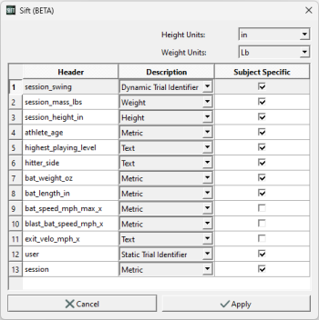
- A metadata dialog box will appear after clicking Create CMZs. Make the following changes in this box:
- Height Units: in
- Weight Units: Lb
- session_swing: Dynamic Trial Identifier
- user: Static Trial Identifier
- Check "Subject Specific" next to highest_playing_level, hitter_side, bat weight/length, and Click "Apply".
- CMZ files may take a while to build. Check the status bar in the bottom left hand corner of the interface for the build status.
Loading Data into Sift
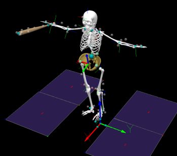
For our analysis, we are interested in finding the variance in pelvic angular velocity between high and low Blast bat speed among college and high school baseball players. For each signal in our analysis, we specified an x, y, and z coordinate for pelvic angular velocity with relation to the virtual lab, expressed in the pelvises coordinate system with movement in the x direction being anterior posterior pelvic tilt, movement in the y direction being lateral pelvic tilt and movement in the z axis being internal external rotation, which can be seen in the image below. Each group was then refined to be categorized into right hitters, competition level (either high school or college), and high or low bat speeds for the subject's specific competition level. If you wish to investigate something new, different approaches can be taken.
Before starting this section of the tutorial please download this .q3d file with premade query definitions.
- Select
 Load Library on the top left corner of the Load page, beside Library Path click on
  Browse, and navigate to the folder where your .cmz and .c3d files are located. Then select Load and exit the window.
 - Navigate to the Explore page and select the
 Query Builder button. Inside the window select Load Query Definitions and navigate to the analysis_of_baseball_hitters.q3d file that you downloaded.
 - Select Calculate All Queries (if you exit the window before the query is fully computed click Compute Groups). Groups will be queried by player level, right hitters, high and low blast bat speeds, and x, y, and z pelvic angular velocity coordinates.
A detailed tutorial on creating groups can be found here. An example of creating a group manually is as follows.
- Select the
 Query Builder button.
 - Add a
 Query (group) and name it “HIGHSCHOOL_RIGHT_LOW_PAV_X”.
 - While the group you just created is selected add a
 Condition and give it the name “highschool_right_low_pav_x”.
- Signals: Type - “LINK_MODEL_BASED” , Folder - “ORIGINAL”, Signal Name - “PEVIS_ANGULAR_VELOCITY”, Component - “X”.
- Refinement:
- Check Refine using tag and select R,
- Check Refine using signal, click
 Add, give it the name “lowBatSpeed”, Type - “METRIC”, Folder - “meta”, Name - “blast_bat_speed_mph_x”, Component - “X”, Value Must Be - “Between”, Min - “57”, Max - “62”, click Save.
 - Click
 Add, give it the name “HIGHSCHOOL”, Type - “TEXT_DATA”, Folder - “meta”, Name - “highest_playing_level”, Component - “X”, Value Must Be - “Equal To”, Value - “high_school”, click Save.
- Once you are happy with your queries click Save Query Definitions to save it as a .q3d file.
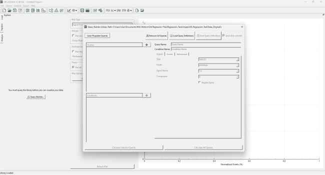
Notes:
- For this tutorial we are basing low and high blast bat speeds off of Blast Motion’s bat speed data based on competition level [5].
- College: low: 61-66 mph, high: 70-73 mph.
- HIGHSCHOOL: low: 57-62 mph, high: 69-71 mph.
Sift Visualization and PCA Analysis
If you haven’t had much experience visualizing signals in Sift, take some time to review the Load and View Data Tutorial.
To begin the PCA (principal component analysis), select two groups that you want to compare. Let's start by looking at HIGHSCOOL_RIGHT_HIGH_PAV_Z and College_RIGHT_HIGH_PAV_Z, select the two groups (CTRL + Click), and check the Select All Workspaces box if it is not already selected.
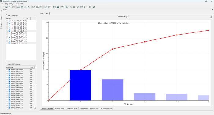
Navigate to the toolbar at the top of the interface and select the ![]() button in the toolbar. Give your PCA a name and select the number of PCs (principal components) you want for your analysis, for this tutorial we will use 5 (more about this in Variance Explained), and then check the Use Workspace Mean if it is not already selected. Now click Run PCA and the graphs will appear in the Analyse page.
button in the toolbar. Give your PCA a name and select the number of PCs (principal components) you want for your analysis, for this tutorial we will use 5 (more about this in Variance Explained), and then check the Use Workspace Mean if it is not already selected. Now click Run PCA and the graphs will appear in the Analyse page.
Once your PCA graph has appeared, at the bottom right of the screen you will see six options for visualizing results of the analysis (variance explained, loading vector, workspace scores, group scores, extreme plot and PC reconstruction).See the Perform Principal Component Analysis for more information on interpreting these results.
Results
We can interpret differences of pelvic angular velocity between different competition levels of hitters through visual comparisons of high blast bat speeds at each coordinate system. Additionally we can analyze the various PCA graphs to look at Variance Explained, Workspace Scores, Group Scores, and Loading Vectors. The aim of this analysis is to assess the impact pelvic angular velocity has on blast bat speeds by comparing high bat speeds between college and high school hitters, and the hypothesis is that hitters at a higher level of competition will have greater pelvic angular velocity subsequently improving their bat speed. Visual comparisons can be a means of illustrating outliers and patterns, whereas PCA can provide statistical verification of whether the two groups accurately reveal disparities from the signals of interest.
Notes:
- The number of college and high school subjects are not balanced, which may lead to inconsistent results between the two groups.
- Examples of interpreting PCA results are shown below and through the following tutorial here.
Visual Comparisons:
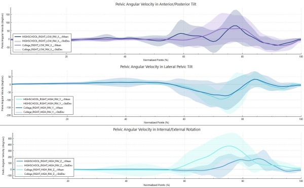
When visualizing different coordinates of the pelvic angular velocity, 3 figures can be laid out in a 3x1 grid. Go to the ![]() Options tab in the toolbar and under Plotting options change Graph Rows to 3, and leave Graph Columns as 1. Selecting one of the graphs will outline it with a gray border, you are then able to select which Groups and Workspaces you would like to display. In the three graphs below we have displayed “HIGHSCHOOL_RIGHT_HIGH_PAV_” and “College_RIGHT_HIGH_PAV_” in their X, Y, and Z coordinates.
Options tab in the toolbar and under Plotting options change Graph Rows to 3, and leave Graph Columns as 1. Selecting one of the graphs will outline it with a gray border, you are then able to select which Groups and Workspaces you would like to display. In the three graphs below we have displayed “HIGHSCHOOL_RIGHT_HIGH_PAV_” and “College_RIGHT_HIGH_PAV_” in their X, Y, and Z coordinates.
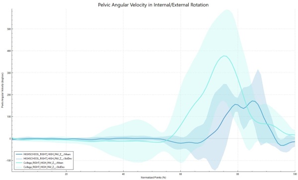
Looking at the anterior/posterior tilt and lateral pelvic tilt graph there is not a large visual difference between our college and high school players. Internal/External Rotation is what we want to focus on, where our college hitters yield a greater peak pelvic angular velocity compared to their high school counterparts. But with that being said, visualizing doesn't always tell the whole story, so let's perform a PCA (Principal Component Analysis) and continue analyzing.
Notes:
- For more details on creating and exporting graphs please take a look at this tutorial here.
Variance Explained:
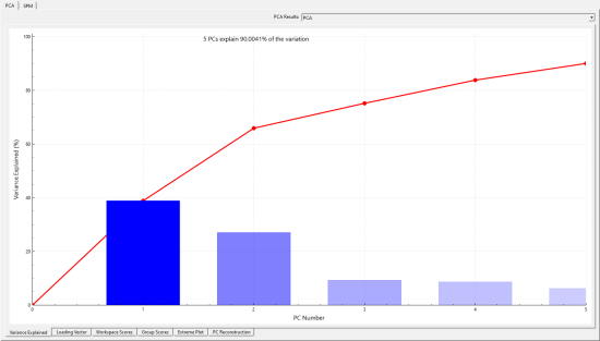
Variance explained is the first graph displayed after running a PCA, and displays the variance explained by each principal component as well as the cumulative variance of each principal component. We can see that 90.0% of the variance can be explained by the first five principal components. Generally you want to increase the number of PCs until they explain 95% of the variance, but for this data set 7 PCs are needed to reach that variance and we don't want to start overfitting or capturing too much noise, so the number of PCs will be left at five.
Group Scores:
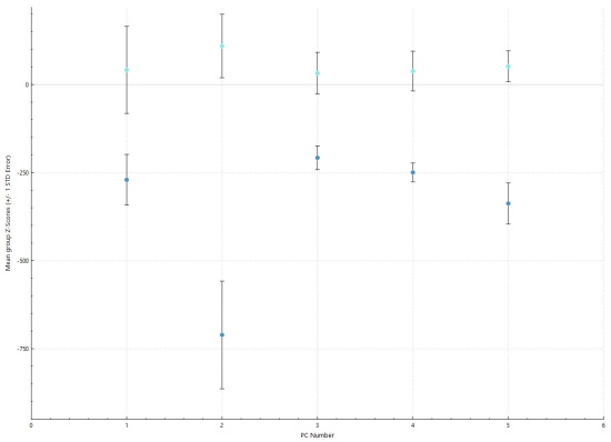
When looking at the group scores the goal is to be able to confidently classify subjects as either being college or high school hitters. Analyzing this graph shows that the standard errors of all five PCs do not overlap, suggesting that all 5 PCs can differentiate between the groups. We can see from variance explained that PC1 accounts for the most overall variation at 38.9%, but since PC2 and PC5 are showing the most significant differences for each group, due to the group scores not overlapping and not crossing over zero they will be the focus of the remaining analysis.
Loading Vector:
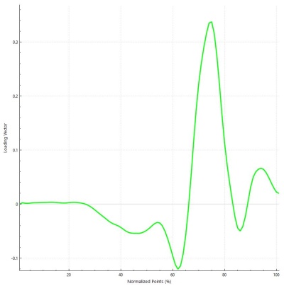
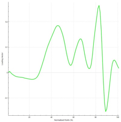
We can take a closer look at PC2 and PC5 to see why these principal components may be showing the most significant differences. Looking at the mean signal trace of the college and high school subjects pelvic internal/external rotation, we can see that the majority of the difference in their swings are at the peak of their pelvic velocity, and also interestingly the high school players have more internal rotation before and at the end of there swing which is represented in PC2. PC5 is less clear and harder to interpret, once again we can see that the high and low points around 80-90 on the x axis are showing the variability between the subjects peak pelvic angular velocity, and the large value around 40 seems to point out that there were more college players with an earlier swing, but the rest is hard to decipher.
Workspace Scores:
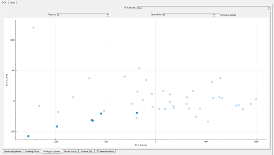
Having identified the principal components of interest, we will switch to the Workspace Scores and plot the chosen PCs against each other (i.e., for this tutorial, plot PC2 versus PC5). We want to be able to distinguish our college group in light blue and high school group in dark blue, and in this graph we can see that there is partial separation between groups. The dark blue high school group seems to be clustered in the bottom left corner with the light blue college group dispersed elsewhere. If there was an even distribution of high school and college subjects (right now there are much fewer high school students) we might have stronger evidence of a relationship between the groups that allows for easier clustering and separation.
Conclusion
From the results of the visual comparisons and the PCA of this tutorial we can conclude that there is a correlation between a high pelvic angular velocity in internal/external rotation and high blast bat speed. This is exemplified by the college hitters exhibiting both a higher pelvic angular velocity and a higher blast bat speed, along with evidence from the PCA that there is a significant level of variability between the two groups.
However, there are limitations on the conclusion such as a disproportionate amount of college subjects compared to high school subjects so the conclusion should be interpreted with caution. This is by no means a complete study and used simply for the demonstration of Sift. Please feel free to explore this data on your own and make improvements while you become comfortable with Sift and its various applications.
References
[1] Wasserberger KW, Brady AC, Besky DM, Jones BR, Boddy KJ. The OpenBiomechanics Project: The open source initiative for anonymized, elite-level athletic motion capture data. (2022). https://www.openbiomechanics.org/
[2] Fortenbaugh, David, "The Biomechanics of the Baseball Swing" (2011). Open Access Dissertations. Paper 540.https://hittingperformancelab.com/wp-content/uploads/2015/01/hitting-baseball-miami-study.pdf
[3] Welch CM, Banks SA, Cook FF, Draovitch P. Hitting a baseball: a biomechanical description. J Orthop Sports Phys Ther. 1995 Nov;22(5):193-201. doi: 10.2519/jospt.1995.22.5.193. PMID: 8580946. https://pubmed.ncbi.nlm.nih.gov/8580946/
[4] Hirano Y. Biomechanical analysis of baseball hitting. In ISBS-Conference Proceedings Archive 1986. https://ojs.ub.uni-konstanz.de/cpa/article/view/1535
[5] Rpp. (2022, February 7). A Review of Blast Motion Baseball and Its Swing Metrics. RPP Baseball. https://rocklandpeakperformance.com/a-review-of-blast-motion-baseball-and-its-swing-quality-metrics/
