Inspect3D Tutorial: Treadmill Walking In Healthy Individuals

Abstract

Visual3D and Inspect3D can be used to automate the processing of large batches of clinical data. This tutorial provides an example of how to do so using a publicly available data set.

Fukuchi et al.[1] published a gold standard public data set [2] of marker-based motion capture to describe healthy individuals walking overground and on a treadmill. Although the authors present a number of descriptive analyses, the effect of using handrail support on gait biomechanics during treadmill walking in this data set has yet to be addressed.

This tutorial is designed to demonstrate how to use Inspect3D to compare joint angles between two groups of older adults: those who used a handrail and those who did not.

Data

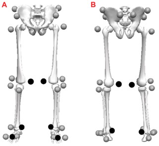
The Fukuchi et al. data set includes 3D kinematic data for 26 lower limb and pelvic markers and ground reaction force plate data for 42 subjects walking at 8 different speeds. Motion capture data was sampled at 150 Hz and force plate data was sampled at 300 Hz. Metadata in these trials included anthropometric measurements such as mass, height, leg length, leg dominance, gender, handrail support, and walking speed. For this tutorial only a subset of the data was used, which included the trials with older adults (subjects 25-42) walking at a single comfortable control speed (T05).

• Fukuchi et. al. subject data: From the publicly available data files, download WBDSc3d.zip for subject .c3d files, and WBDSinfo.xlsx for the metadata [3]

To simplify this tutorial, the following premade files are available to download as a starting point. They are contained in the zip folder labelled "I3D_Tutorial_Treadmill_Walking.zip", which can be downloaded here. The file types and contents are briefly described below:

• Visual3D Workspaces (processed_workspaces): Pre-processed .cmz and .c3d files for the elderly subject group (subjects 25-42). Contains pre-made tags (see Table 1).

• Visual3D Pipeline (pipeline.v3s): Compiles the static and motion .c3d files, associates them with a model file, and sets premade tags for all of the participants in this dataset. The pipeline produces separate .cmx and .cmz files for each participant.

• Model Template (WBDSmodel.mdh): Provided by Fukuchi et. al. Includes lower body and pelvis segments generated using the 26 anatomical markers, and is applied to the subject .c3d files. If you wish to build your own model, follow the Model Building Tutorial.

• Query Definitions (group_definitions.q3d): Query definitions for Inspect 3D loading X, Y, and Z components of lower body joint angles, with signals not combined across sides of the body.

• Inspect3D Workspace (workspace.i3d): Copy of working Inspect3D workspace.

• Inspect3D Color Palette (FukuchiPalette.xml): Premade color template used for generating images in this tutorial.

Table 1 below shows the tags used in this tutorial. These will be used in later steps.

Table 1: Tag Definitions

Tag	Definition
SLOW, CONTROL, FAST	Walking speeds.
YOUNG, OLD	Subject age.
MALE, FEMALE	Subject sex.
LEFTDOMINANT, RIGHTDOMINANT	Subject leg dominance.
HELDRAIL	Subject held rail during treadmill walking trial.
DIDNOTHOLDRAIL	Subject did not hold rail during treadmill walking trial.

Visual3D Processing

If you want to skip to the Inspect3D analysis portion of this tutorial, ensure you have downloaded the "I3D_Tutorial_Treadmill_Walking.zip" folder and then skip to the header called Loading Data into Inspect3D. If you want to use or modify the pre-made pipeline, continue with the steps below. You also need to have downloaded the original data from Fukuchi et al.[4]

This tutorial uses the Pipeline feature of Visual3D to process the raw data provided by Fukuchi et al. The benefit of the pipeline feature is that it can be used to automate repeated steps and reduces the amount of time it takes to work with large data sets. If you are unfamiliar with using the Visual3D workspace, take some time to review the Typical Processing Session Tutorial and the Command Pipeline Tutorial.

1. Download .c3d files: Fukuchi et al. has a folder labelled WBDSc3dWithGaitEvents, ensure that you are using the .c3d files contained in this folder.

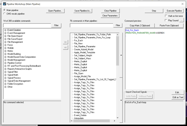
2. Subject by Subject Pipeline Edits: If you haven't yet, download "pipeline.v3s" from "I3D_Tutorial_Treadmill_Walking.zip". This pipeline compiles all the static and dynamic .c3d files, associates them with a model file, and sets tags for all of the subjects, then generates separate .cmx and .cmz files for each subject. You can open the pipeline in a text editor and search and edit these functions manually, or open the Pipeline Workshop and edit them in the Visual3D interface. This pipeline must be run once for each subject, with the following changes being made before each run:

• Subject Index: Under pipeline function Set_Pipeline_Parameter, change PARAMETER_VALUE to the value associated with each subject (01, 02, 03...).
• Subject Height: Under pipeline function Set_Subject_Height, change the HEIGHT parameter to match the subject. Height is in cm.
• Subject Mass: Under pipeline function Set_Subject_Mass, change the WEIGHT parameter to match the subject. Weight is in kg.
• Subject Age: Under pipeline function Explicit_Metric, there should be a parameter called RESULT_METRIC_NAME set to ISOLD. Set to 1 if subject is older than 50 and 0 if subject is under 50.
• Subject Gender: Under pipeline function Explicit_Metric, there should be a parameter called RESULT_METRIC_NAME set to ISMALE. Set to 1 if subject is male and 0 if subject is female.
• Subject Foot Dominance: Under pipeline function Explicit_Metric, there should be a parameter called RESULT_METRIC_NAME set to ISLEFTDOMINANT. Set to 1 if subject is left footed and 0 if subject is right footed.
• Subject Rail Use: Under pipeline function Explicit_Metric, there should be a parameter called RESULT_METRIC_NAME set to HELDRAIL. Set to 1 if subject used the rail and 0 if the subject did not use the rail.

This information is contained in the metadata file mentioned previously.

3. Load and Execute Pipeline: Open Visual3D and click on the "Pipeline" button on the toolbar at the top of the interface. Select "Open Pipeline" and navigate to the directory where you saved the subject specific version of pipeline.v3s. Click "Open" and "Execute Pipeline". The pipeline script will prompt you to select a folder path. Choose the location of the .c3d files referenced in instruction 1. The pipeline loads the static trial and treadmill dynamic trails for a subject. Ensure that your model template file is in the same folder as your static and motion files, or you will be prompted to select the model for each subject that is processed in the pipeline. The script will apply the model to the motion files, add tags to the appropriate files, modify force plate parameters, clean force assignments and compute gait events, and compute signals for link model based measures of interest. A .cmz file is produced for each participant at the end of the pipeline.

4. Verify Execution: Check that .cmz and .cmx files were created for each subject.

5. Repeat for all desired subjects.

Loading Data into Inspect3D

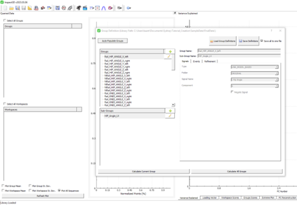
Within the "I3D_Tutorial_Treadmill_Walking.zip" folder there is a subfolder labelled "processed_workspaces". This contains the Visual3D workspaces that must be loaded into Inspect3D for further analysis.

1. Select Load Library and set CMO Library Path to the folder where your .cmz and .c3d files are located. Ensure you are using the files from the WBDSc3dWithGaitEvents folder. Then select Load and exit the window.
2. Open the Group Definitions tab and select Load Group Definitions. Once prompted, open the group_definitions.q3d query file.
3. Select Calculate All Groups. Groups will be divided up based on right and left pelvis, hip, knee and ankle joint angles in x, y, and z axis.

A detailed tutorial on creating groups can be found here. An example of creating a group manually is as follows.

1. Open the Group Definitions Dialog.
2. Add a group and name it “Rail_HIP_ANGLE_X_right”
3. Add a sub-group and name it “Rail_HIP_ANGLE_X_right”
   1. Signals: Type - “LINK_MODEL_BASED”, Folder - “ORIGINAL”, Signal Name - “L Hip Angle”, Component - “X”
   2. Events: Event Sequence - LHS,LHS
   3. Refinement: Select Refine using tag, and Use and Logic, Highlight HELDRAIL and CONTROL

For our investigation, we are interested in comparing railing holding to non railing holding while walking on the treadmill. For each signal in our analysis, we specified which railing condition we wanted, and used the control speed (trial T05 of treadmill data in raw data files). For our investigation we specifically looked at the effect of holding rails, however, if you wish to investigate something new, different tags can be selected.

Cleaning Data

If you haven't had much experience cleaning data in Inspect3D, take some time to review the Clean Your Data Tutorial.

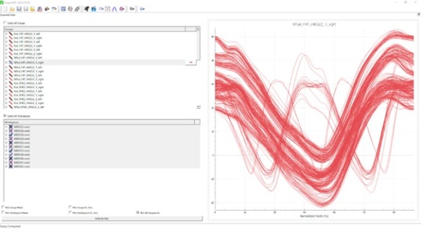
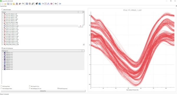
To begin cleaning your data, start by selecting a group to graph, then clicking Select all Workspaces and then Plot all Sequences. On the plotted graph, select any traces you wish to inspect. Right click on the graph and hover over Exclude, then click Exclude Trace (raw data). In the toolbar select Update CMZs to update the files with the excluded traces.

Depending on how you clean your data, results may vary.

Inspect3D Visualization and PCA Analysis

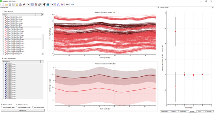
If you haven't had much experience visualizing signals in Inspect3D, take some time to review the Load and View Data Tutorial.

To start a PCA analysis, start by selecting the two groups you want to compare in the Groups menu (CTRL + Click). Example: CTRL + Click on Rail_Pelvis_Angle_Y and NRail_Pelvis_Angle_Y.

Navigate to the toolbar at the top of the interface and select the button. A dropdown menu will appear. Select the number of PCAs you want for your analysis and ensure Use Workspace Mean is checked. Then click Run PCA and Show PCA Graphs. The PCA graph should appear on the right side of the user interface

Once the PCA has been run, at the bottom right corner of the Inspect3D interface there are six options for visualising results of the analysis (variance explained, loading vector, workspace scores, group scores, extreme plot and PC reconstruction). See the Perform Principal Component Analysis for more information on using these tools and interpreting results.

Results

Interpretation of joint angle signals can be made through visual comparison of the two study groups: hand railing support and non-hand railing support during control speed treadmill walking. Additionally, waveform-based PCA can help us find differences in the waveform data between the two study groups. The goal of this analysis is to determine if the joint angles of the lower body are affected by the use of hand-rails during treadmill walking. Visual comparison can be used to depict outliers and pattern behaviour, whereas PCA can provide statistical verification of whether two groups can be distinctly identified from the signals of interest.

Examples of interpreting PCA results are shown below in the knee, hip, and pelvis, and through the following tutorial here.

Ankle

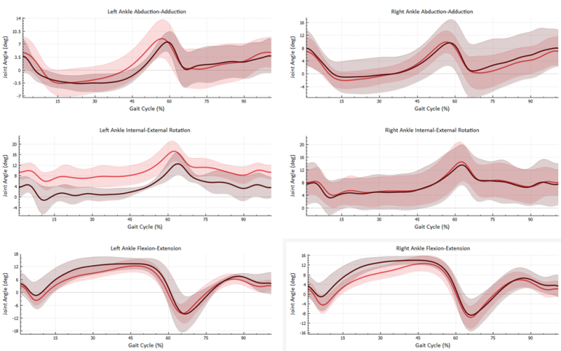
For this study, to look specifically at one joint 6 figures can be laid out in a 3x2 grid. To do so go to the Options tab and change the number of rows and columns. This allows for easy comparison between the different angle changes in different directions. We plotted the left and right ankle angles in abduction-adduction, internal-external rotation, and flexion-extension to compare signals between railing and non-railing walking conditions. Visual analysis showed very similar trajectories over a gait cycle, however holding the railing (dark red) appeared to have greater variability during stance for left angle in abduction-adduction and internal-external rotation. For the right leg they overall show similar trajectories.

Knee

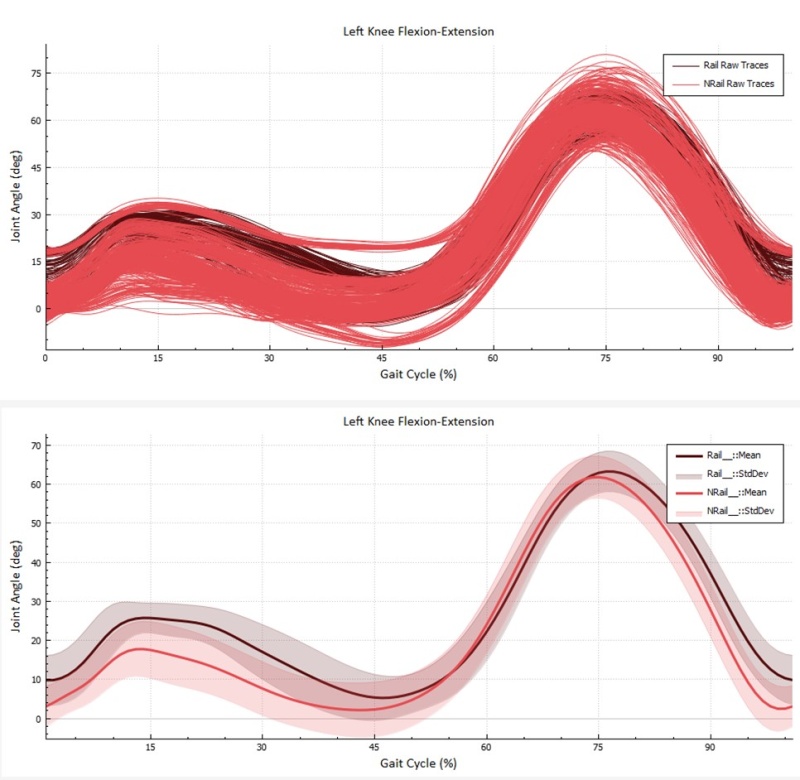
We plotted the left knee angle signals over a gait cycle, including the mean and standard deviations for both railing and non-railing groups. For the coordinate system used in the Fukuchi et. al. data set, the Z-axis is aligned in the medial/lateral direction, and so the knee angle about the Z-axis describes the flexion/extension rotation. In this analysis, we can see that there is some amount of distinction in the mean values between those holding a railing, and those not holding a railing, particularly during stance (0-45%) and late-swing phase (90%+). It appears that those holding the rail had a higher mean joint angle in both those instances.

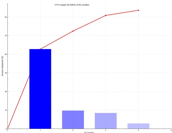
We then performed a PCA analysis on the knee data. Through this we can see that the underlying gait cycle signal is structured, and 95% variance can be explained by the first four principal components.

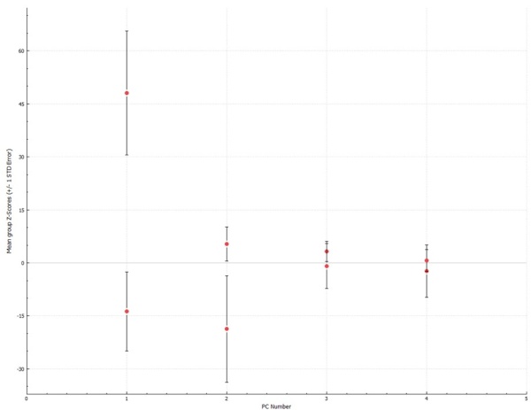
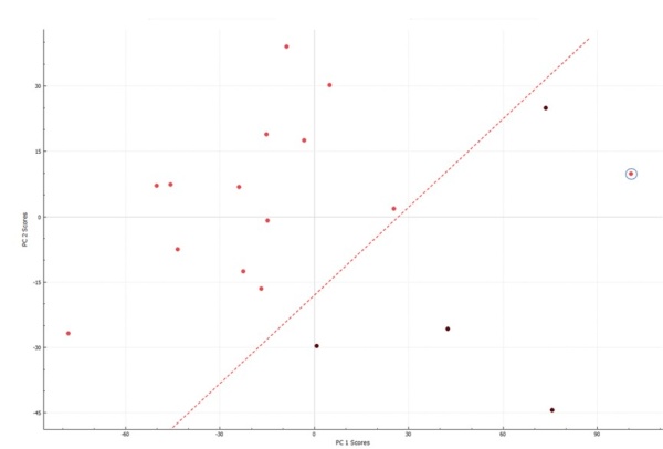
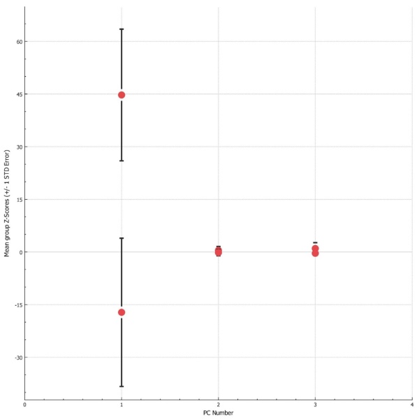
Returning to our visualisation analysis on the knee, we know that there are potential differences between the knee angles of those who used the railing, and those who did not. If possible, we want to be able to classify subjects as having used the railing, and not having used it. By looking at the Group Scores tab, that is the average values of each principal component on each group, we see that the standard errors of PC1 and PC2 do not overlap, suggesting PC1 and PC2 can best discriminate between groups. PC4 for example, has standard errors that do overlap, signifying that it could not be used to discriminate the groups. We can graph both PC1 and PC2 through the Workspace Scores tab, and see that we have a nearly linearly separable dataset.

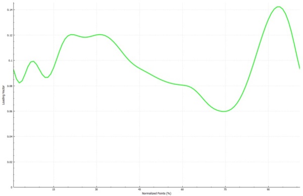
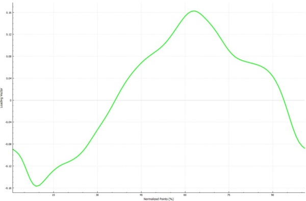
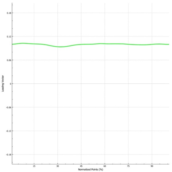
We can then look more closely at PC1 and PC2, and see why this may make sense. Looking back at the mean signal trace graph, we see that there is a notable difference in the joint angle between the 2 groups at the beginning and end of the gait cycle, and PC1 in particular may represent this. We can see by plotting the vector of PC1 that in general, the value of PC4 is smaller in the middle, while it is a large value at both the beginning and end of the gait cycle. Since we can visually see that the subjects who held the rail generally had higher angles at these points in the cycle, we would expect, and in fact do see, large values of PC1. While this is not a perfect separation of the two groups, the addition of PC2 explains the variance, again at the very start where we see the most difference, and around 60-75% where there is slight variance.

Hip

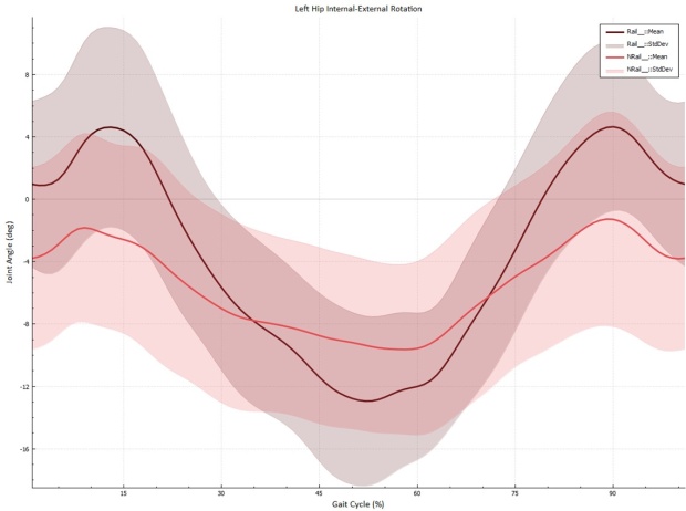
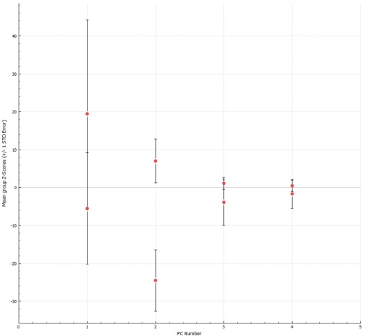
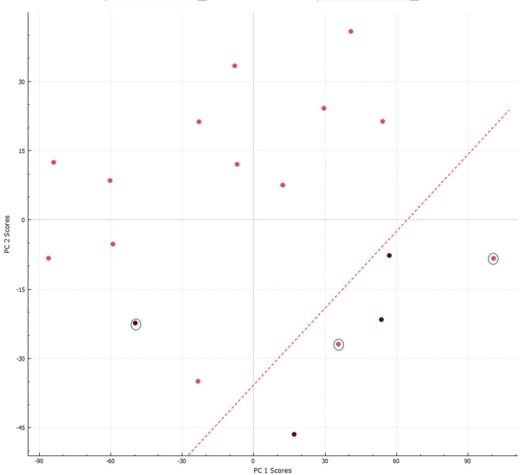
We plotted the left hip internal and external rotation over a gait cycle, including the mean and standard deviations for both railing and non-railing groups. For the coordinate system used in the Fukuchi et. al. data set, the Y-axis is aligned in the vertical direction, and so the hip angle about the Y-axis describes internal-external rotation behaviour. Using Inspect3D’s PCA analysis, we plotted the Group Scores tab for the first 4 principal components that described >95% of the hip joint signals, with the mean and standard error. We found that the second principal component has identifiable differences in the scores between groups, as the standard errors do not cross the x-axis. Further investigation into this principal component using the Workspace Scores we can see a reasonable separation between groups when comparing PC2 to PC1. In this specific example, PC1 describes more of the dataset variability for each group (64.1%), however, PC2 can best discriminate between the compared groups when analysing the hip internal-external rotation.

Pelvis

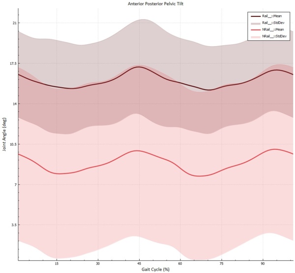
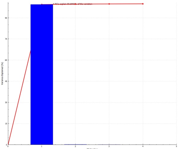
When comparing pelvis angles during the gait cycle, we noticed variations in the Z-axis behaviour. For the coordinate system used in the Fukuchi et. al. data set, the Z-axis is aligned in the medial/lateral direction, and so rotation about this axis defines the anterior-posterior rotation of the pelvis. We can see directly from plotting mean and standard deviation of the group signals, the non-railing condition appears to have much greater variability across those subjects. The mean signal trajectory shows that the subjects who did not hold the railing were walking with a more upright pelvis position, and those who did hold the railing walked with a greater forward tilt in the lower trunk/pelvis. Moving to our PCA analysis, we can see that almost 100% of the variability between group signals can be described by PC1, and PC1 can also be used to discriminate between signals when analysing anterior/posterior pelvis angle.

Conclusions

The quantitative results for the lower limb joint PCA analyses are summarized below in Table 2. The ankle analysis had unreliable data and was therefore excluded from the results table.

Table 2: PCA Results

Joint	PC of Significance	% of Variance Explained by Significant PC	% of Variance Explained by 4 PCs
Knee Flexion-Extension	PC1	64.1%	95%
Hip Internal-External Rotation	PC2	16.4%	98%
Anterior-Posterior Pelvic Tilt	PC1	99.99%	99%

From these results we can conclude that holding a hand rail does have the statistical potential to influence lower limb joint angles (particularly the pelvic angle) and should be a variable that is controlled for in future studies.

However, there are limitations on the conclusions that can be drawn from this analysis. Firstly, eliminating the younger subjects from the analysis pool reduced the subject pool from 42 to 17. This number of subjects is typically acceptable for pilot studies but is not large enough to be statistically valid for the general population. Secondly, to further quantify the relationship between rail use and lower limb joint angles it would be more effective to have the same subjects walk with and without a handrail (which was not the case in this data set). This would better control for variations in individual gait patterns.

References

Data set: Fukuchi et al. A public dataset of overground and treadmill walking kinematics and kinetics in healthy individuals: [5]

Paper: Fukuchi et al. A public dataset of overground and treadmill walking kinematics and kinetics in healthy individuals: [6]

License: Original Dataset is licensed under CC BY 4.0 [7]